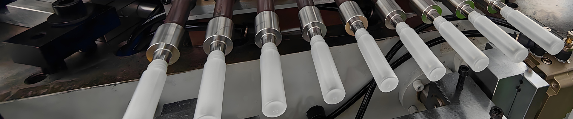
Cycle time reduction is the single most powerful output lever available to an injection blow molding plant, because every second removed from the cycle multiplies across every cavity, every shift, and every operating day of the machine’s life. On a three-station one-step IBM machine running eight cavities, trimming a 12.8 second cycle to 10.4 second lifts gross hourly output by more than 23 percent without adding a single square meter of floor space, a single operator, or a single mold. Aibim, a Wanplas factory with 12 years of machine building experience, a dedicated CNC center for critical machine parts, a new plant purchased in 2022 with capacity for more than 100 machines per year, and installations in over 40 countries, designs its IBM55 Hybrid, IBM65, and IBM75 platforms specifically around this arithmetic. This guide breaks the IBM cycle into its measurable phases, explains the physics that sets the hard floor on cooling time, presents ten field-proven acceleration levers with realistic gains and quality risks, and closes with a structured implementation method that protects wall thickness uniformity, weight consistency, clarity, and neck dimensional tolerance while the numbers on the counter go up.
The critical discipline is that speed and quality are not opposites, but they are coupled. Almost every acceleration lever has a quality metric it can damage if pushed past its safe boundary. A plant that shortens cooling by three seconds and ships deformed bottles has not gained output; it has converted good parts into scrap and moved the bottleneck from the machine to the inspection table. For that reason, every recommendation below is paired with a boundary criterion, a measurable indicator that tells the process engineer when the lever has reached its limit. The goal is not the shortest possible cycle. The goal is the shortest cycle that holds a process capability index at or above 1.33 on the critical dimensions, sustained over a full production campaign.
لماذا زمن الدورة هو الرافعة الرئيسية لربحية IBM
In injection blow molding, cycle time governs output, unit energy consumption, labor absorption, and the effective payback of the capital equipment simultaneously. Unlike changes to material grade or mold cavitation, which usually require validation, tooling investment, or customer approval, a cycle improvement earned through machine and process tuning is available immediately and applies to every part number that runs on the machine.
الإنتاج يتدرج خطيًا، وأكثر من ذلك
Gross output in pieces per hour equals 3,600 divided by cycle time in seconds, multiplied by cavity count. An eight-cavity tool at 12.0 second delivers 2,400 pieces per hour gross; the same tool at 10.0 second delivers 2,880 pieces per hour, a gain of 480 pieces every hour. Across three shifts and 300 operating days, that difference approaches 3.5 million additional containers per year from equipment that is already installed and already staffed. This is why an experienced IBM plant treats a 0.5 second improvement as a serious engineering win rather than a rounding error.
يتم تخفيف التكاليف الثابتة
A significant share of an IBM plant’s cost base is time-based rather than piece-based: operator wages, plant depreciation, facility heating and lighting, compressed air standby, chiller base load, and quality staff. Every one of these is spread across more pieces when the cycle shortens. The relative cost category of an individual container therefore moves from Medium toward Low as cycle time falls, even though nothing about the raw material or the machine has changed.
موثوقية التسليم وسعة الطلبات
Cycle time is also a commercial weapon. A plant with a 15 percent faster cycle can quote shorter lead times, accept rush orders, and hold buffer capacity for seasonal peaks in cosmetics and pharmaceutical packaging. In competitive tendering for pharmaceutical bottle contracts, the ability to guarantee a monthly volume with headroom is frequently the deciding factor, ahead of marginal differences in the price of the container.
استقرار الدورة لا يقل أهمية عن طول الدورة
A machine that averages 11.0 second but varies between 10.2 and 12.4 second is harder to plan and produces more dimensional variation than a machine that holds 11.4 second with a standard deviation below 0.15 second. Variation in cycle time means variation in melt residence time, variation in cooling contact duration, and therefore variation in shrinkage and neck dimensions. Any cycle reduction program must therefore track both the mean and the spread, and must reject a change that shortens the average while widening the distribution.
تحليل دورة IBM: تفصيل كامل للمراحل
You cannot shorten what you have not measured, and in a three-station one-step IBM machine the measurement is more subtle than in a straight injection molding machine because three stations work in parallel while the index and clamp events are strictly sequential. The total cycle equals the sequential events plus the longest of the three parallel station windows. Understanding this structure immediately reveals which levers pay and which do not.
الأحداث المتتابعة مقابل نافذة المحطة المتوازية
On the standard three-station layout, station one performs parison injection onto the core rod, station two performs blowing in the blow mold, and station three strips the finished container. All three happen at the same time. When the slowest station finishes, the clamp opens, the turntable indexes 120 degrees, the clamp closes and locks, and the next window begins. Therefore the machine cycle is: clamp close plus parallel window plus clamp open plus index plus handshake confirmation. Any second removed from a station that is not the slowest station produces zero improvement in cycle time. This single insight prevents a great deal of wasted optimization effort.
يفكك الجدول أدناه دورة زمنية تمثيلية مدتها 12.0 ثانية لزجاجة تجميل من HDPE سعة 100 مل بثمانية تجاويف وبجدار اسمي 1.1 مم، تعمل على آلة IBM هيدروليكية متوسطة الحجم. النسب المئوية هي حصص من إجمالي الدورة البالغة 12.0 ثانية.
| Cycle segment | Type | Typical duration (s) | Share of cycle (%) | Bottleneck potential |
|---|---|---|---|---|
| Clamp close and lock build-up | Sequential | 0.50 | 4.2 | Low |
| Parallel station window (longest station governs) | Parallel | 9.00 | 75.0 | Very High |
| Clamp open to safe index height | Sequential | 0.50 | 4.2 | Low to Medium |
| Turntable index, 120 degree rotation and settle | Sequential | 1.20 | 10.0 | Medium to High |
| Strip confirmation and part clearance signal | Sequential | 0.40 | 3.3 | Low |
| Interlock handshake and dry return idle | Sequential | 0.40 | 3.3 | Medium |
| Total cycle | — | 12.00 | 100.0 | — |
ما الذي يحدث داخل نافذة التوازي البالغة 9.0 ثانية
The parallel window is where three quarters of the cycle lives, so it deserves its own decomposition. The table below shows what each of the three stations does inside that same window. Notice that station three sits idle for most of the window, and that station one and station two are both dominated by cooling. This is the classic IBM signature: the bottleneck is almost never injection or blowing, it is heat removal.
| Station | Sub-phase | Duration (s) | Share of the 9.0 s window (%) | Runs in parallel with |
|---|---|---|---|---|
| 1 الحقن | Parison fill, multi-stage velocity | 1.20 | 13.3 | Blow at station 2 |
| 1 الحقن | Pack and hold to gate freeze | 1.60 | 17.8 | Blow hold at station 2 |
| 1 الحقن | Parison cooling on core rod after gate freeze | 6.20 | 68.9 | Screw plasticizing, blow mold cooling |
| 1 الحقن | Screw plasticizing (fully overlapped) | 5.50 | 61.1 | Parison cooling, must stay shorter |
| 2 Blow | Blow mold contact and seal | 0.40 | 4.4 | الحقن fill |
| 2 Blow | Preblow, low pressure expansion | 0.50 | 5.6 | الحقن fill |
| 2 Blow | Final blow and pressure hold | 1.40 | 15.6 | Pack and hold at station 1 |
| 2 Blow | Blow mold cooling with air exchange | 6.30 | 70.0 | Parison cooling at station 1 |
| 2 Blow | Exhaust and pressure release | 0.40 | 4.4 | End of window |
| 3 Strip | Container stabilization before release | 1.80 | 20.0 | Everything |
| 3 Strip | Stripper actuation and discharge | 0.80 | 8.9 | Everything |
| 3 Strip | Idle waiting for the slowest station | 6.40 | 71.1 | Free capacity |
قراءة نقطة الاختناق بشكل صحيح
In the example above, station two governs the window at approximately 9.0 second, driven almost entirely by blow mold cooling at 6.3 second. Station one is close behind at 9.0 second, dominated by 6.2 second of parison cooling on the core rod. Station three has 6.4 second of spare time. The conclusion is unambiguous: any effort spent making the stripper faster, or making the injection fill faster, returns essentially nothing, while every 0.1 second removed from either cooling stage returns 0.1 second of real cycle. That is where engineering attention belongs.
كيفية التقاط هذه الأرقام على آلة حقيقية
Most modern IBM controllers can display a phase timing screen or export a shot log. Where that is unavailable, a two-person manual method works: one engineer records the controller phase timers over 50 consecutive shots while a second uses a handheld timer on the visible mechanical events, specifically clamp open start, index start, index end, and clamp lock. Averaging 50 shots removes operator reaction error. Record the mean and the standard deviation for each segment, and build the two tables above for your own machine before changing anything. Plants that skip this step almost always tune the wrong phase.
مرجع الدورة الجافة
Every IBM machine has a dry cycle time, the time required to complete clamp close, index, and clamp open with no material and no cooling. On a well-maintained mid-size hydraulic IBM machine this is typically 2.4 to 3.0 second, and on a hybrid servo-driven machine it can fall to 1.8 to 2.4 second. The dry cycle is the mechanical floor of the machine. If your production cycle is 12.0 second and your dry cycle is 2.6 second, then 9.4 second is process time, and process time is where the opportunity lies. If, on the other hand, your dry cycle has drifted from 2.6 second to 3.6 second because of worn guides, low accumulator pressure, or slow valve response, then you have a maintenance problem masquerading as a process problem.
السقف الفيزيائي: زمن التبريد وقانون مربع سماكة الجدار
Cooling time in injection blow molding is not a setting the operator chooses freely; it is a physical quantity governed by heat conduction through the polymer wall, and it obeys a square law with respect to thickness. Understanding this relationship tells a process engineer exactly how much cycle is theoretically available and prevents wasted effort chasing gains that physics will not allow.
العلاقة الحاكمة
For one-dimensional conduction through a plastic wall cooled from both sides, the required cooling time scales as the square of the wall thickness divided by the thermal diffusivity of the polymer. In compact form, cooling time is proportional to s squared divided by alpha, where s is wall thickness and alpha is thermal diffusivity. A logarithmic term accounts for the melt temperature, the mold surface temperature, and the target demolding temperature, but that term changes slowly, while the thickness term changes quadratically. Thickness therefore dominates everything.
ما يعنيه قانون المربع عمليًا
Because the relationship is quadratic, a 10 percent reduction in wall thickness produces roughly a 19 percent reduction in cooling time, since 0.9 squared equals 0.81. A 20 percent thickness reduction produces about a 36 percent cooling reduction. Conversely, a designer who adds 15 percent wall for stiffness has silently added 32 percent to the cooling requirement and destroyed a large part of the plant’s output plan. This is why wall thickness is the first item to review whenever a new bottle drawing arrives, and why cycle time must be discussed at the design review, not after tooling is cut.
| Nominal wall thickness (mm) | Relative cooling time index (1.0 mm = 100) | Change versus 1.0 mm baseline | Practical note for IBM containers |
|---|---|---|---|
| 0.50 | 25 | Minus 75 percent | Very thin cosmetic and sample vials; blow uniformity becomes the limit |
| 0.60 | 36 | Minus 64 percent | Thin-wall eye drop and diagnostic containers |
| 0.80 | 64 | Minus 36 percent | Standard small pharmaceutical bottle wall |
| 1.00 | 100 | Baseline | Common reference for 50 to 200 ml containers |
| 1.20 | 144 | Plus 44 percent | Typical cosmetic bottle requiring squeeze resistance |
| 1.50 | 225 | Plus 125 percent | Heavy chemical or rigid closure-mounted containers |
| 2.00 | 400 | Plus 300 percent | Thick-wall specialty parts; cycle becomes cooling dominated |
الانتشارية الحرارية حسب المادة
The second variable in the cooling equation is the effective thermal diffusivity of the polymer, which bundles thermal conductivity, density, and specific heat, and for semi-crystalline resins also absorbs the latent heat of crystallization. A material with higher effective diffusivity gives up heat faster and allows a shorter cooling stage at the same wall thickness. The values below are typical engineering figures for process estimation; confirm against the resin supplier datasheet for the specific grade before committing to a production cycle.
| Material | Typical effective thermal diffusivity (mm squared per second) | Melt temperature window (degrees C) | Typical demolding temperature (degrees C) | Relative cooling demand at equal wall |
|---|---|---|---|---|
| HDPE | 0.10 to 0.12 | 180 to 230 | 60 to 75 | Medium |
| LDPE and LLDPE | 0.11 to 0.13 | 170 to 215 | 50 to 65 | Medium |
| PP homopolymer | 0.065 to 0.095 | 200 to 250 | 70 to 90 | High |
| PS general purpose | 0.085 to 0.095 | 190 to 240 | 65 to 80 | Medium to High |
| SAN | 0.085 to 0.100 | 210 to 250 | 75 to 90 | Medium to High |
| ABS | 0.095 to 0.110 | 210 to 250 | 75 to 90 | Medium |
| PC | 0.120 to 0.135 | 280 to 320 | 115 to 130 | Medium, but high melt temperature extends the term |
| PCTG and PETG | 0.085 to 0.100 | 230 to 260 | 60 to 75 | High |
| TPU | 0.080 to 0.095 | 190 to 225 | 40 to 55 | Very High, soft demolding limit |
لماذا تتصرف الراتنجات شبه البلورية بشكل مختلف
البولي بروبيلين and polyethylene release latent heat as they crystallize, which effectively lowers their apparent diffusivity during the phase change and lengthens the cooling stage relative to what a simple conduction calculation predicts. البولي بروبيلين is the more difficult of the two because its crystallization proceeds over a wider temperature range and its parts remain soft at temperatures where polyethylene has already stiffened. This is exactly the situation where a nucleating agent pays back, a point developed later in this guide.
مصطلح درجة الحرارة وتأثيره المحدود
The logarithmic term in the cooling relationship contains the melt temperature, the mold surface temperature, and the demolding temperature. Lowering the mold surface temperature by 5 degrees C shortens cooling time by a few percent, not tens of percent, and it carries the risk of surface defects, reduced clarity in amorphous resins, and increased molded-in stress. Melt temperature has a similar limited leverage, and reducing it too far raises injection pressure and risks incomplete parison filling. Temperature is therefore a fine-tuning variable in a cycle program, not a primary lever. The primary levers are wall thickness, heat transfer efficiency in the tool, and the removal of non-cooling time from the cycle.
عشر أدوات مجربة لتقليل زمن دورة IBM
The following ten levers cover the realistic field toolkit for reducing injection blow molding cycle time. Each is presented with the practical action, the typical achievable gain, the quality metric it can damage, and the conditions under which it applies. The summary table appears first for planning purposes, followed by the engineering detail for each lever.
| # | Lever | Typical cycle gain | Primary quality risk | Applies when |
|---|---|---|---|---|
| 1 | Core rod and mold cooling circuit optimization | 8 to 18 percent | Local overcooling, gate freeze too early, short shot | Cooling dominates the parallel window |
| 2 | Mold temperature controller and chiller matching | 5 to 12 percent | Condensation, surface haze, dimensional drift | Supply to return delta T exceeds 4 degrees C |
| 3 | Multi-stage injection velocity and V-P switchover tuning | 4 to 8 percent | Flash, jetting, weight variation, sink marks | Fill plus hold exceeds 3.0 second |
| 4 | Plasticizing fully parallel to cooling | 0 to 10 percent | Unmelted particles, melt temperature rise, degradation | Plasticizing time approaches or exceeds cooling time |
| 5 | Back pressure and screw speed rebalancing | 2 to 6 percent | Shear degradation, color streaking, melt overheating | Plasticizing is the constraint inside station one |
| 6 | Hot runner balancing across cavities | 3 to 7 percent | Cavity-to-cavity weight spread, short shot in lean cavities | Weight coefficient of variation above 1.5 percent |
| 7 | Servo index drive instead of hydraulic index | 5 to 10 percent | Parison sag during transfer, core rod alignment wear | Index time exceeds 1.6 second |
| 8 | Clamp motion profiling and minimum safe stroke | 3 to 6 percent | Mold face impact, safety interlock margin loss | Clamp open plus close exceeds 1.4 second |
| 9 | Blow air timing compression and exhaust sizing | 3 to 8 percent | Incomplete cavity contact, wall thinning, burst | Blow plus exhaust exceeds 2.4 second |
| 10 | Take-out and discharge motion overlap | 2 to 5 percent | Container deformation while still warm, scuffing | Station three is the governing station |
Gains are not additive. A plant that applies all ten levers typically realizes 18 to 30 percent total cycle reduction from an untuned baseline, not the arithmetic sum, because each improvement exposes the next constraint. Work in order of the measured bottleneck, re-measure after each change, and stop when the marginal gain no longer justifies the quality risk.
الرافعة 1: تحسين قضيب اللب ودائرة تبريد القالب
This is the highest-yield lever in injection blow molding because the core rod is simultaneously the parison-forming surface, the transfer carrier, and the primary heat sink on the inner wall. A core rod with a single central bore and a return annulus removes heat unevenly along its length, leaving the shoulder region hot and forcing the whole cooling stage to wait for the slowest zone. Replacing that arrangement with a properly proportioned bubbler or a multi-channel design equalizes the surface temperature and shortens the governing cooling stage.
Three quantitative targets govern circuit design. First, the coolant flow must be turbulent, not laminar: the Reynolds number in each circuit must exceed 4,000, and a target of 6,000 to 10,000 gives a comfortable margin. Turbulent flow can improve the heat transfer coefficient by a factor of three to five compared with laminar flow at the same coolant temperature, which is why a plant that merely opens the water valve wider often gains more than one that buys a bigger chiller. Second, channel bore should be sized so that the pressure drop across the circuit stays manageable while turbulence is maintained; 8 to 10 mm bores are common for blow mold body circuits and 4 to 6 mm for core rod bubblers. Third, the distance from the channel wall to the molding surface should be roughly one to one and a half times the channel diameter, and the pitch between adjacent channels should be roughly two to three times the diameter, so that the cooling front is even rather than scalloped.
Conformal cooling, in which the channel follows the contour of the molding surface rather than being drilled in straight lines, is increasingly practical for core rods and blow mold inserts produced by additive manufacturing or by brazed insert construction. On a shouldered cosmetic bottle where a straight-drilled circuit leaves a hot band at the shoulder radius, a conformal insert can remove that hot band entirely and cut two to three seconds from the governing cooling stage. The relative investment category is High, but on a high-volume long-life tool the payback in output is substantial.
The quality risk is local overcooling. If the circuit near the gate becomes too aggressive, the gate freezes before packing is complete, producing sink marks, low weight, and a rise in weight variation. The boundary criterion is straightforward: monitor part weight and its coefficient of variation while shortening cooling. When the coefficient of variation begins to climb above 1.0 percent, or when weight drops by more than 0.5 percent, the cooling has begun to interfere with packing.
الرافعة 2: مطابقة جهاز التحكم في درجة حرارة القالب والمبرّد (Chiller)
Many IBM plants run an undersized or mismatched thermal system and never realize it. The rule is that the chiller and mold temperature controller together must remove the heat the process puts in, at a supply to return temperature difference small enough to keep the mold surface uniform. A large temperature difference between supply and return means the coolant is heating up as it travels, so the downstream half of the circuit is cooling less effectively than the upstream half, producing dimensional gradients across the container.
The design target is a supply to return delta T of 2 to 3 degrees C on blow mold circuits and no more than 3 degrees C on core rod circuits. If measured delta T exceeds 4 degrees C, increase flow rate before lowering supply temperature. Lowering supply temperature to compensate for insufficient flow is a common error: it increases the risk of condensation on the mold face in humid plants, it raises molded-in stress, and it can produce surface haze on amorphous resins, while doing little to fix the underlying non-uniformity.
Sizing the refrigeration capacity requires a simple heat balance. The heat to be removed equals the mass throughput of polymer multiplied by the specific enthalpy change from melt temperature to demolding temperature. For polyolefins, a practical planning figure is roughly 0.30 to 0.40 kW of refrigeration capacity per kilogram per hour of throughput, plus an allowance for hydraulic oil cooling and ambient gain. A machine molding 60 kg per hour of HDPE therefore needs roughly 18 to 24 kW of process cooling for the tool, plus separate capacity for the hydraulic circuit. Undersizing here caps every other lever, because no amount of injection tuning will help if the tool cannot shed heat.
The quality risk is condensation and thermal shock. The boundary criterion is the plant dew point: mold surface temperature must remain above the dew point of the workshop air, otherwise water films on the mold face will cause surface marks and, over time, corrosion of the tool. Where a low mold temperature is genuinely needed in a humid climate, dehumidified enclosure air or a dry air purge on the mold face is the correct answer.
الرافعة 3: سرعة الحقن متعددة المراحل وضبط تبديل V-P
Parison injection in IBM is not a single-speed event. A well-built profile uses a moderate speed through the gate to avoid jetting, a fast fill through the parison body to keep the melt front hot and uniform, and a controlled deceleration before the parison is complete so that the switchover from velocity control to pressure control happens without a pressure spike. Getting this profile right shortens fill time and, more importantly, shortens the required hold time because a uniformly filled parison needs less packing to compensate for uneven density.
The switchover position is the critical parameter. Set it too early and the machine relies on holding pressure to complete the fill, which is slow and produces weight variation. Set it too late and the machine reaches the end of stroke under velocity control, generating a pressure spike that causes flash at the parting line and stresses the tool. The classic method is to fill at velocity to approximately 95 to 98 percent of the shot volume and let holding pressure complete the last few percent. Confirm the position by producing a short-shot series with holding pressure at zero: the correct switchover position gives a parison that is 95 to 98 percent complete.
A four-stage profile is usually sufficient for IBM parisons: slow through the gate region, fast through the main body, medium through the shoulder transition, slow into the switchover. Typical achievable gains are 0.3 to 0.6 second from fill and hold combined. The quality risks are jetting and flash if the profile is too aggressive, and short shot or sink if the switchover is too early. The boundary criteria are visual inspection for jetting patterns near the gate, parting line inspection for flash, and part weight stability across 30 consecutive shots.
الرافعة 4: التلدين بالتوازي الكامل مع التبريد
In a well-configured IBM machine, the screw recovers the next shot while the current parison cools on the core rod. This overlap is free cycle time, and it is available only if the plasticizing time is genuinely shorter than the cooling time. When plasticizing takes longer than cooling, plasticizing becomes the governing constraint inside station one, and every second of cooling improvement you achieve is wasted because the machine is waiting for the screw.
The diagnostic is simple: read the plasticizing time and the cooling time from the controller. Plasticizing should finish with at least a 15 to 20 percent time margin before cooling ends. If plasticizing occupies 5.5 second inside a 6.2 second cooling stage, the margin is only 11 percent, and a further cooling reduction of one second would make the screw the bottleneck. In that situation the correct sequence is to first shorten plasticizing, then shorten cooling.
Shortening plasticizing without damaging the melt means raising screw speed moderately, reducing back pressure to the minimum that still gives a homogeneous melt and a stable cushion, verifying that the barrel temperature profile is not so conservative that the screw is doing all the melting by shear, and confirming that the check ring and screw tip are not worn. A worn non-return assembly leaks melt backward during injection, which the controller compensates for by extending recovery, so a plasticizing time that has crept upward over months is frequently a wear signal rather than a settings problem.
The quality risk is unmelted particles and melt temperature rise. The boundary criteria are melt temperature measured with a probe in an air shot, which should stay inside the grade’s recommended window, and visual inspection of the parison for unmelted specks or streaking. If melt temperature rises more than 8 to 10 degrees C above the target when screw speed is increased, the shear input is excessive and the barrel profile should be adjusted instead.
الرافعة 5: إعادة موازنة الضغط الخلفي وسرعة اللولب
Back pressure and screw speed are the two knobs that determine both melt quality and recovery time, and they pull in opposite directions. High back pressure improves melt homogeneity, drives out entrapped air, and stabilizes the shot size, but it lengthens recovery and raises melt temperature through shear. High screw speed shortens recovery but reduces residence time for melting and can generate localized shear heating.
For most IBM applications on polyolefins, a back pressure in the range of 3 to 8 bar of specific melt pressure is sufficient. Plants frequently run 15 to 20 bar out of habit inherited from engineering-resin injection molding, which needlessly extends recovery. Reducing excessive back pressure is one of the cheapest cycle gains available, requiring nothing but a controller change and a verification run. Screw speed should be set so that the peripheral screw speed stays within the grade’s shear tolerance; for standard polyolefin IBM grades a peripheral speed of 0.15 to 0.35 meters per second is a safe working band.
The quality risks are shear degradation, color streaking in pigmented resin, and shot size instability if back pressure falls too low. The boundary criterion is cushion stability: the cushion must remain constant within roughly 0.3 mm across 30 shots. If the cushion begins to wander when back pressure is reduced, the melt is not consolidating properly and the reduction has gone too far.
الرافعة 6: موازنة المجرى الساخن عبر التجاويف
In a multi-cavity IBM tool, cavity-to-cavity imbalance forces the process engineer to run the whole tool at the settings required by the worst cavity. If one cavity fills slightly late, holding pressure must be extended for every cavity so the lean one packs out. That extra hold time is pure cycle waste applied to seven or eleven perfectly good cavities.
Balancing starts with measurement: run a short-shot series and weigh each cavity individually, then compute the coefficient of variation of cavity weights. A well-balanced IBM tool holds cavity weight variation below 1.0 percent; above 1.5 percent there is meaningful cycle time trapped in the imbalance. Correction options in order of increasing effort are individual hot runner zone temperature trimming, gate land adjustment, flow channel rebalancing, and manifold rework. Zone temperature trimming alone can often bring a 2.0 percent spread down to 1.0 percent, and each 0.5 percentage point of improvement typically allows 0.15 to 0.3 second of hold time to be removed.
The quality risk is that trimming one zone to fix a lean cavity can overheat that zone’s melt, causing color shift or degradation in heat-sensitive grades. The boundary criterion is that no zone should be trimmed more than 10 to 15 degrees C from the nominal manifold setting; if a larger correction is needed, the imbalance is mechanical and must be fixed in the flow channel, not with heat.
الرافعة 7: محرك فهرسة سيرفو بدلاً من الفهرسة الهيدروليكية
The 120 degree turntable index is a purely sequential event, which makes it a high-value target: every 0.1 second removed from the index is 0.1 second removed from the cycle, with no parallel activity to absorb it. A conventional hydraulic index with a rack-and-pinion or rotary actuator arrangement typically requires 1.8 to 2.6 second including acceleration, deceleration, and settle time, because hydraulic motion is hard to profile precisely and needs generous deceleration to avoid slamming the index stops.
A servo-driven index with a closed-loop position profile typically completes the same 120 degree rotation in 1.0 to 1.4 second. The servo can accelerate hard, cruise, and decelerate on a controlled S-curve into the locking position without overshoot, and it repeats that profile within a few milliseconds shot after shot. On a 12.0 second cycle, moving from a 2.2 second hydraulic index to a 1.2 second servo index removes 1.0 second, an 8.3 percent cycle reduction from a single subsystem.
| Index drive characteristic | Conventional hydraulic index | Servo-driven index | Effect on cycle |
|---|---|---|---|
| Typical 120 degree index time | 1.8 to 2.6 s | 1.0 to 1.4 s | 0.6 to 1.2 s direct saving |
| Shot-to-shot index repeatability | Plus or minus 60 to 120 ms | Plus or minus 5 to 20 ms | Lower cycle standard deviation |
| Motion profile control | Valve and flow restriction based | Programmable S-curve, closed loop | Less settle time required |
| الطاقة draw during index | Pump running at pressure throughout | Current drawn only while moving | Lower energy per cycle |
| Alignment repeatability at station lock | Depends on mechanical stops | Encoder verified position | Less core rod wear over time |
| Parison sag exposure during transfer | Longer transfer, more sag risk | Shorter transfer, less sag | Better wall uniformity at speed |
The quality risk of a fast index is parison disturbance. The parison is still hot and deformable while it rotates on the core rod, and an aggressive acceleration profile can induce sag or ovality, which shows up as wall thickness asymmetry in the blown container. The boundary criterion is wall thickness measurement around the circumference at three heights; if circumferential variation grows beyond the tolerance band as index acceleration is increased, soften the acceleration ramp while keeping the higher cruise speed.
الرافعة 8: تشكيل حركة الإغلاق وأدنى شوط آمن
Clamp open and clamp close are sequential events that together typically occupy 1.0 to 1.6 second. Two adjustments shorten them. First, motion profiling: the clamp should move fast through the free travel and slow only in the final approach where mold protection is active. Many machines are set with a conservative low-speed segment far longer than necessary, often because the profile was never revisited after the tool was commissioned. Second, stroke minimization: the open stroke needs to be only as large as required to clear the tallest container plus the core rod plus a safety margin. Reducing an over-generous open stroke by 40 mm on a toggle clamp can save 0.15 to 0.3 second per cycle.
Aibim’s single-crossbeam, double-pole clamping framework with enlarged mold setting space helps here in a practical way: the enlarged daylight means the tool designer does not need to compromise, and the operator does not need to run an oversized stroke to accommodate awkward mold geometry. Combined with the PREFILL hydraulic technology, which pre-charges the clamp actuator so the pump does not have to move full oil volume against pressure during the low-load part of the stroke, the clamp completes its fast travel with less pump work and less time.
The quality and safety risk is mold face impact and loss of interlock margin. Never reduce the low-speed mold protection segment below the distance in which the machine can detect an obstruction and stop. Aibim machines are CE certified with a long-distance digital laser sensor at the stripper station for mold safety and a light curtain for personnel safety; these systems must retain their full detection window regardless of any speed tuning. The boundary criterion is a documented mold protection test: place a soft obstruction in the mold area and verify the machine stops without damage at the tuned speed.
الرافعة 9: ضغط توقيت هواء النفخ وتحديد حجم العادم
The blow sequence consists of preblow at low pressure, transition to final blow at high pressure, a pressure hold while the container contacts the cavity wall, and exhaust. Compressing this sequence is worthwhile when blow plus exhaust exceeds roughly 2.4 second. Three specific measures deliver most of the gain.
First, tighten the preblow to final blow transition. Preblow exists to start the expansion gently so the wall distributes evenly; once the container has taken shape, delaying the high-pressure switch adds nothing. Advancing the switch point by 0.1 to 0.2 second is often available with no wall thickness penalty. Second, reduce the pneumatic dead volume. The air between the valve and the blow pin must be pressurized and then vented every cycle; shortening the hose run, moving the valve closer to the blow pin, and eliminating unnecessary fittings reduces both the pressurization time and the exhaust time. Third, size the exhaust valve properly. An undersized exhaust port can add 0.3 to 0.5 second to every cycle simply because the container cannot depressurize quickly enough to allow safe mold opening. Increasing exhaust bore is usually a low-cost modification with an immediate return.
A further refinement is exhaust air recovery, in which the depressurizing air from the high-pressure blow stage is routed into the low-pressure preblow reservoir rather than vented to atmosphere. This does not shorten the cycle by itself, but it reduces compressor load, which stabilizes the supply pressure and therefore makes the blow timing more repeatable at high output rates.
The quality risks are incomplete cavity contact, localized wall thinning, and burst. The boundary criteria are full detail reproduction on the container surface, wall thickness within tolerance at the base and shoulder, and a burst pressure test result that retains at least the specified safety margin over the intended filling and capping pressures.
الرافعة 10: تداخل حركة الإخراج والتفريغ
Station three, the stripper station, usually has spare time, but on very short cycles or with tall containers it can become the governing station. When that happens, the fix is motion overlap: begin the stripper approach while the clamp is still completing its opening stroke, and begin the discharge conveyor motion while the stripper is retracting, rather than running these motions strictly one after another. On machines with a take-out robot or a chute with an air assist, the discharge can be fully overlapped with the index.
The limit is container stability. A container stripped too early is still above its heat distortion temperature in the thickest sections and will deform under the stripper’s contact force or under its own weight in the discharge chute. The boundary criterion is a dimensional check on containers taken from the discharge point rather than from the mold: measure neck ovality and body diameter on 20 pieces after they have cooled to ambient. If the discharge-point sample shows greater deviation than a hand-caught sample cooled without contact, the container is being handled too hot.
السرعة مقابل الجودة: مصفوفة المفاضلة والحدود الآمنة
Every acceleration lever borrows from a quality reserve, and the discipline of a professional cycle reduction program is knowing exactly which reserve is being spent and how much remains. The matrix below pairs each lever with the quality characteristic most likely to degrade, the physical mechanism behind the degradation, and a measurable boundary criterion that signals when to stop.
| Acceleration action | الجودة metric at risk | Mechanism | Safe boundary criterion |
|---|---|---|---|
| Shorten parison cooling on core rod | Wall thickness uniformity, shoulder ovality | Parison still soft at transfer, sags during index | Circumferential wall variation stays inside the drawing tolerance at three measured heights |
| Shorten blow mold cooling | Demolding deformation, base push-up, panel distortion | Container above heat distortion temperature when released | Body diameter after 24 hours stays within tolerance; no base rocker |
| Reduce holding time | Part weight, weight coefficient of variation, sink marks | Gate not yet frozen, melt back-flows out of the parison | Weight coefficient of variation below 1.0 percent across 30 shots |
| Increase injection velocity | Flash at parting line, jetting near gate, burn marks | Pressure spike at switchover, trapped gas compression heating | No visible flash at nominal clamp force; no jetting pattern on cut sections |
| Lower mold temperature to speed cooling | Clarity and gloss in amorphous resins, molded-in stress | Frozen skin layer, higher orientation locked into the wall | Haze value and stress crack resistance meet the product specification |
| Increase screw speed to shorten plasticizing | Melt homogeneity, color consistency, degradation | Insufficient residence time, excess shear heating | Melt temperature rise below 8 to 10 degrees C; no specks or streaking |
| Reduce back pressure | Shot size stability, entrapped air, surface bubbles | Melt not consolidated, air carried into the parison | Cushion stable within 0.3 mm across 30 shots |
| Accelerate turntable index | Wall asymmetry, core rod and bushing wear | Inertial deformation of the hot parison, mechanical shock | Wall asymmetry unchanged from baseline; no rise in index position error |
| Compress blow timing | Cavity detail reproduction, neck finish dimensions, burst strength | Insufficient contact time against the cavity wall | Neck thread and sealing surface within tolerance; burst test margin retained |
| Overlap stripping with clamp motion | Container deformation, scuffing, neck ovality | Handling while sections are above heat distortion temperature | Discharge-point sample matches hand-caught sample dimensionally |
| Raise regrind percentage to lower cost | Cycle stability, weight drift, clarity | Variable bulk density and thermal history alter feeding and melting | Cycle standard deviation stays below 0.20 second; weight drift below 0.5 percent per hour |
تشطيب الرقبة هو أصعب قيد
Among all quality metrics affected by cycle acceleration, the neck finish deserves special attention because injection blow molding’s principal advantage over extrusion blow molding is precisely that the neck is injection molded to close tolerance with no flash and no trimming. A cycle reduction that compromises neck dimensions gives away the reason the customer chose injection blow molding in the first place. Neck thread pitch, sealing surface flatness, inner diameter, and perpendicularity should be measured on a sample of at least 20 containers before and after every significant cycle change, and any statistically detectable shift should be treated as a rejection of that change until the cause is understood.
الإجهاد المتبقي: العيب الذي يظهر لاحقاً
Faster cooling and lower mold temperature both increase frozen-in orientation and residual stress. The danger is that this defect frequently does not appear at the machine. It appears weeks later as environmental stress cracking in a filled bottle in a warehouse, particularly with surfactant-containing cosmetic or household chemical contents in polyethylene containers. Any cycle program that reduces cooling significantly should include an accelerated stress test on the final container with the intended contents, not just a dimensional check at the machine. This is standard practice for pharmaceutical and personal care packaging and should not be skipped in the pursuit of output.
تأسيس حد أدنى للجودة قبل البدء
Define the quality floor in writing before the first setting is changed. A workable floor for most IBM containers includes: part weight within plus or minus 2 percent of nominal with a coefficient of variation below 1.0 percent; wall thickness within the drawing tolerance at all measured points; neck critical dimensions with a process capability index of at least 1.33; no visible flash, jetting, sink, or haze defect above the agreed limit sample; and a leak test pass rate of 100 percent on the sampled population. With this floor documented and agreed with quality assurance, cycle reduction becomes an engineering exercise with a clear stopping rule rather than a negotiation between production and quality.
تقليل الدورة من ناحية المواد: التدفق والتنوي وإعادة الطحن
Machine and tooling levers are only half the picture. The polymer itself sets limits on how fast the parison can be filled, how quickly it gives up heat, and how stable the cycle remains over a long run. Material selection is often the fastest route to a shorter cycle because it requires no capital expenditure, though it does require validation with the customer for regulated packaging.
درجات أعلى لمعدل تدفق الذوبان
A higher melt flow rate grade fills the parison at lower pressure and lower melt temperature, and the lower melt temperature directly shortens the cooling requirement because there is less heat to remove. Moving from a 4 gram per 10 minute HDPE to an 8 gram per 10 minute HDPE typically allows a 5 to 10 degrees C reduction in melt temperature at the same fill time, which translates into roughly 3 to 6 percent less cooling time. The trade-off is mechanical: higher flow grades have lower molecular weight, which reduces environmental stress crack resistance and top-load strength. For a rigid cosmetic bottle this is often acceptable; for a container holding an aggressive chemical it may not be.
| Material | Typical IBM grade melt flow rate (g per 10 min) | Effect of moving to the higher end of the range | Property to verify before switching |
|---|---|---|---|
| HDPE | 2 to 12 | Lower melt temperature, 3 to 6 percent cooling reduction | Environmental stress crack resistance, top load |
| LDPE and LLDPE | 4 to 20 | Faster fill on thin walls, easier small container filling | Squeeze recovery, drop impact |
| PP homopolymer | 10 to 40 | Significant fill improvement, allows thinner walls | Impact strength at low temperature, clarity |
| PP random copolymer | 8 to 30 | Better clarity retention with good flow | Stiffness, heat resistance for hot filling |
| PS general purpose | 4 to 16 | Very easy filling of thin decorative containers | Brittleness, crazing resistance |
| SAN | 5 to 15 | Improved detail reproduction on textured surfaces | Chemical resistance to fragrance oils |
| PC | 8 to 25 | Lower melt temperature reduces the long cooling term | Notch sensitivity, hydrolytic stability, drying |
| PCTG and PETG | Grade specific, viscosity rated | Reduced injection pressure, less shear whitening | Clarity, chemical resistance, drying discipline |
عوامل التبلور للبولي بروبيلين
البولي بروبيلين is the material most often responsible for a disappointing IBM cycle, because it crystallizes slowly and remains soft well below its melting point. A nucleating agent supplies crystal initiation sites throughout the melt so that crystallization begins at a higher temperature and completes faster. The practical consequence is that the container reaches a demoldable stiffness sooner, allowing the cooling stage to be shortened.
Typical results with a well-dispersed nucleating agent at normal addition levels include a crystallization temperature increase of 8 to 15 degrees C, a cooling time reduction of 10 to 20 percent, improved dimensional stability because post-mold shrinkage is reduced, and higher stiffness at equal wall thickness, which sometimes allows a further thickness reduction and a second round of cooling gain through the square law. Clarifying nucleating agents additionally improve transparency in random copolymer polypropylene, which matters for cosmetic and diagnostic containers. The cost category of the additive is Medium, but the output gain is usually decisive on a high-volume line.
Two cautions apply. First, dispersion quality determines the result; poorly dispersed nucleating masterbatch produces localized crystallization differences and can worsen warpage. Second, for pharmaceutical and food contact containers the additive must be compliant with the applicable food contact and pharmacopeia requirements in the target market, and the change must go through the customer’s change control process.
إعادة الطحن واستقرار الدورة
Regrind directly affects cycle time stability rather than cycle length. Ground material has a different bulk density and particle geometry than virgin pellets, which changes the feeding behavior at the screw and therefore changes recovery time shot to shot. It also carries a prior thermal history, so its viscosity is not identical to virgin material. The result is a wider distribution of plasticizing time and, at high regrind levels, a wider distribution of part weight.
| Regrind content | Typical effect on cycle standard deviation | Typical effect on part weight spread | Recommended control measure |
|---|---|---|---|
| 0 percent, virgin only | Baseline, below 0.10 s achievable | Coefficient of variation below 0.6 percent | Standard process control |
| Up to 10 percent | Little measurable change | Coefficient of variation below 0.8 percent | Consistent grinder screen size, dust removal |
| 10 to 20 percent | Slight widening, 0.10 to 0.18 s | Coefficient of variation 0.8 to 1.2 percent | Gravimetric blending rather than volumetric |
| 20 to 30 percent | Noticeable widening, 0.18 to 0.30 s | Coefficient of variation 1.2 to 1.8 percent | Gravimetric blending plus regrind drying and metal separation |
| Above 30 percent | Cycle instability likely, above 0.30 s | Coefficient of variation above 1.8 percent | Not recommended for tolerance-critical necks |
Because injection blow molding produces no tail flash and no pinch-off scrap, the regrind stream in an IBM plant is normally limited to startup shots and rejected containers, which is a considerable inherent advantage over extrusion blow molding. This means an IBM plant can usually stay below the 10 percent regrind band where cycle stability is essentially unaffected, and that in turn makes a tight, fast, repeatable cycle easier to hold.
انضباط التجفيف يحمي الدورة
Hygroscopic materials such as PC, PCTG, PETG, and some SAN grades must be dried to the supplier’s specified residual moisture before molding. Inadequate drying causes splay, bubbles, and viscosity variation, and the variation in viscosity translates into variation in fill and hold behavior, which forces the process engineer to add safety margin to the cycle. Correct drying is therefore not only a quality measure but a cycle measure, because a stable melt viscosity is what allows the hold time to be trimmed to its true minimum.
منهجية التنفيذ: خط الأساس والتجارب و SPC وإجراءات التشغيل القياسية
ينجح برنامج تقليل الدورة أو يفشل على أساس المنهجية، وليس الذكاء. التسلسل خماسي المراحل أدناه هو البنية التي يستخدمها مهندسو Aibim أثناء التشغيل وأثناء تشخيصات الدورة في الموقع، ويعمل بشكل جيد أيضًا لمصنع يحسّن خطًا قائمًا.
المرحلة 1: قياس خط الأساس عبر 50 حقنة متتالية
Record 50 consecutive cycles without changing anything. For each shot capture total cycle time, fill time, hold time, cooling time, plasticizing time, index time, clamp open and close times, cushion, and part weight for at least one designated reference cavity. Compute the mean and standard deviation of each. This baseline serves three purposes: it identifies the governing station and the governing phase, it establishes the natural variation of the process so that later improvements can be distinguished from noise, and it provides the before column of the final comparison table.
Fifty shots is the practical minimum. Fewer than 30 gives an unreliable standard deviation; more than 100 rarely adds information for this purpose. Capture the data at steady state, at least 45 minutes after startup, with the same operator, same material lot, and same ambient conditions, so that the baseline reflects normal running rather than a warm-up transient.
المرحلة 2: تجارب متغير واحد
Change one variable at a time, in a defined step, and hold everything else constant. The temptation to change three settings at once is strong when production pressure is high, but it destroys the ability to attribute the result and makes rollback impossible. A workable trial protocol is: change one variable, run 20 shots to purge the transient, then record 30 shots of data, then evaluate against both the cycle target and the quality floor. If the change passes, keep it and move to the next variable. If it fails, revert immediately and record why.
Step sizes matter. For cooling time, steps of 0.3 to 0.5 second are appropriate; smaller steps are lost in noise and larger steps risk a sudden quality failure that contaminates the next several shots. For injection velocity, steps of 10 percent of the current setting work well. For back pressure, steps of 1 to 2 bar of specific melt pressure are sufficient. For index acceleration, work in 10 percent increments and watch wall symmetry closely.
المرحلة 3: تأكيد الحالة المستقرة
A setting that works for 30 shots does not necessarily work for 30 minutes. Thermal equilibrium in the tool shifts as the shorter cycle changes the heat input rate, and the mold surface temperature may drift upward or downward over the first 20 to 40 minutes after a cooling change. Always run a confirmation period of at least 60 minutes at the new setting, and re-measure part weight, wall thickness, and neck dimensions at the end of it. Many apparently successful cycle reductions fail at this stage, and finding that out in a controlled trial is far better than finding it out in a production run.
المرحلة 4: التحكم الإحصائي في العمليات مع هدف قدرة
Once the new cycle is confirmed, move the critical characteristics onto a control chart. The recommended set is part weight, neck inner diameter, neck sealing surface height, body wall thickness at the thinnest measured point, and total cycle time. Sample at a defined frequency, typically five pieces every hour for a stable process. The acceptance target is a process capability index of at least 1.33 on each dimensional characteristic, which corresponds to a comfortable margin between the natural process spread and the specification limits.
If a characteristic sits between 1.00 and 1.33 after the cycle reduction, the process is producing conforming parts but has lost its safety margin, and a single disturbance such as a material lot change will produce rejects. In that situation, give back a portion of the cycle gain until the capability index recovers. A cycle that is 0.4 second longer and statistically capable is more profitable than a faster cycle that generates sorting, re-inspection, and customer complaints.
المرحلة 5: التقييس وقفل الوصفة
An improvement that is not documented will be lost at the next changeover. Write the confirmed parameter set into a standard operating procedure that includes the full parameter list, the tool and material it applies to, the measured baseline and improved cycle, the quality floor and how to verify it, and the name of the engineer who validated it. Then lock the recipe in the machine controller. Aibim machines include an SD card parameter storage system that lets a validated recipe be saved and reloaded, and moved to a second machine running the same tool family, so the improvement transfers across the plant rather than living in one operator’s memory.
قبل وبعد: نتيجة ممثلة
The table below shows a realistic outcome for an eight-cavity 100 ml HDPE cosmetic bottle program after a structured application of the levers described in this guide. Output figures use the same availability and quality assumptions in both columns except where the improvement itself changed them. Financial values are expressed as index points rather than currency.
| Metric | Before the program | After the program | Change |
|---|---|---|---|
| Total cycle time | 12.80 s | 10.40 s | Minus 18.8 percent |
| Cycle standard deviation | 0.34 s | 0.13 s | Minus 62 percent |
| Governing station | Station 2, blow mold cooling | Station 1, parison cooling | Bottleneck shifted |
| Index time | 2.20 s hydraulic | 1.20 s servo | Minus 1.00 s |
| Plasticizing margin inside cooling | 11 percent | 24 percent | Constraint removed |
| Gross output, 8 cavities | 2,250 pcs per hour | 2,769 pcs per hour | Plus 23.1 percent |
| Availability | 88.0 percent | 90.0 percent | Plus 2.0 points |
| الجودة yield | 97.5 percent | 98.2 percent | Plus 0.7 points |
| Good output per hour | 1,930 pcs | 2,447 pcs | Plus 26.8 percent |
| Good output per 8 hour shift | 15,440 pcs | 19,576 pcs | Plus 4,136 pcs |
| Neck inner diameter capability index | 1.41 | 1.38 | Retained above the 1.33 target |
| Part weight coefficient of variation | 0.82 percent | 0.74 percent | Improved with better balance |
| OEE index, baseline equals 100 | 100 | 127 | Plus 27 index points |
Note that the quality yield improved rather than degraded. This is a common and initially counter-intuitive result: a program that removes cycle variation, balances the cavities, and fixes the thermal system usually produces a more consistent container than the slower, sloppier process it replaced. Speed obtained through better control is not the enemy of quality; speed obtained by simply turning down the cooling timer is.
آلات الحقن والنفخ من Aibim للأعمال عالية الإنتاج
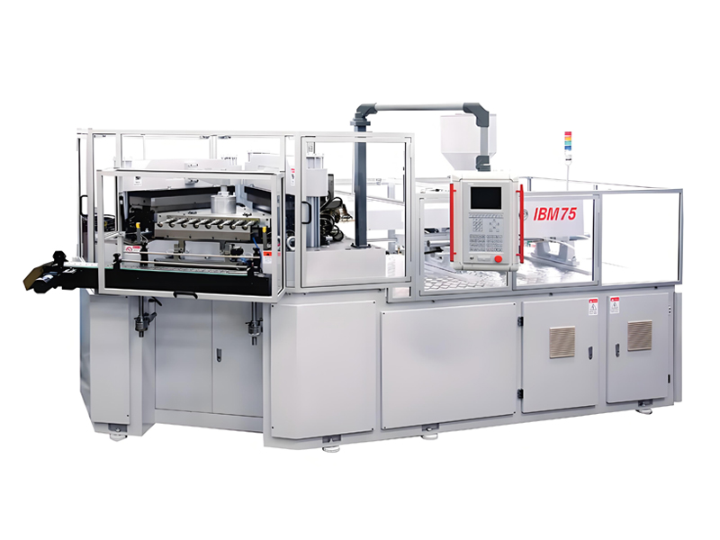
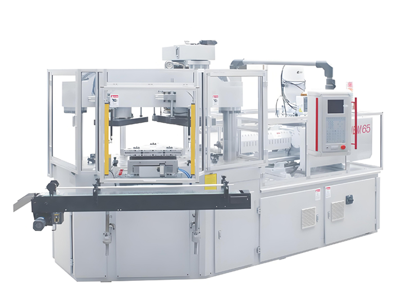
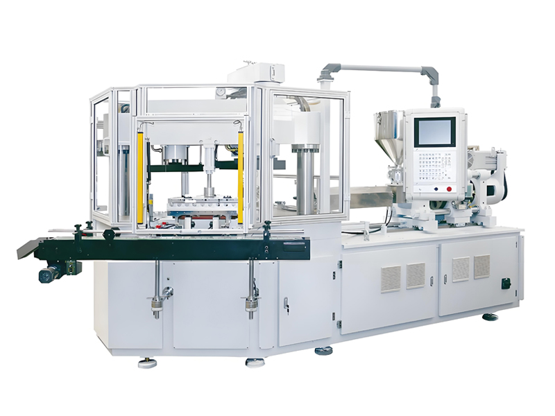
Aibim is a Wanplas factory in Zhangjiagang dedicated to three-station one-step injection blow molding machines and molds, with more than 12 years of machine manufacturing experience, an in-house CNC center for critical machine parts, a plant acquired in 2022 with an annual capacity of more than 100 machines, and installations in over 40 countries. All three machine series share the design features that matter most for cycle time: the PREFILL hydraulic technology and variable displacement pump pressurizing system that reduce pump work and shorten clamp and injection motions, the single-crossbeam double-pole clamping framework with enlarged mold setting space that allows generous cooling circuit routing in the tool, CE certified safety with a long-distance digital laser sensor at the stripper station and a light curtain for personnel protection, SD card parameter storage that transfers a validated fast-cycle recipe from one machine to another, and a verified minimum 35 percent energy saving versus conventional hydraulic equipment. The specification ranges below are typical engineering windows; confirm exact figures against the factory datasheet for your specific mold and material.
آلة القولبة بالنفخ بالحقن IBM75
The IBM75 is the largest of the three series and is the correct choice when container volume reaches the 200 to 1000 ml range or when a thicker wall makes cooling the dominant constraint. Its larger shot capacity and clamping force allow a mold with generous cooling circuit cross-section, which is precisely what a cycle reduction program needs on heavier containers.
| Parameter | Typical value or range |
|---|---|
| Model | IBM75 |
| Process | Three-station one-step injection blow molding |
| الحقن screw diameter | 45 mm |
| Shot size | 80 to 150 g |
| Clamping force | 750 kN |
| Container volume range | 50 to 1000 ml |
| Typical cavity count | 4 to 8 depending on container size |
| Production cycle time | 10 to 16 s |
| وقت دورة التجفيف | 2.6 to 3.0 s |
| Index time, 120 degrees | 1.2 to 1.8 s configuration dependent |
| Installed power | 25 to 33 kW |
| Hydraulic system | PREFILL technology with variable displacement pump pressurizing |
| Drive option | Hydraulic with servo index available |
| الطاقة saving versus conventional hydraulic | Minimum 35 percent |
| Processable materials | HDPE, LDPE, LLDPE, PP, PS, ABS, SAN, TPU, PC, PCTG |
| Parameter storage | SD card recipe save and reload |
| Safety | CE certified, laser sensor at stripper station, light curtain |
آلة القولبة بالنفخ بالحقن IBM65
The IBM65 is the volume workhorse for pharmaceutical and cosmetic containers between roughly 10 and 500 ml, where cavity counts of eight to twelve are common and the cycle target usually sits between 9 and 14 second. It offers the best balance of cavitation, cycle speed, and footprint for the majority of small-container programs.
| Parameter | Typical value or range |
|---|---|
| Model | IBM65 |
| Process | Three-station one-step injection blow molding |
| الحقن screw diameter | 40 mm |
| Shot size | 60 to 110 g |
| Clamping force | 650 kN |
| Container volume range | 10 to 500 ml |
| Typical cavity count | 8 to 12 depending on container size |
| Production cycle time | 9 to 14 s |
| وقت دورة التجفيف | 2.4 to 2.8 s |
| Index time, 120 degrees | 1.1 to 1.6 s configuration dependent |
| Installed power | 18 to 25 kW |
| Hydraulic system | PREFILL technology with variable displacement pump pressurizing |
| Drive option | Hydraulic with servo index available |
| الطاقة saving versus conventional hydraulic | Minimum 35 percent |
| Processable materials | HDPE, LDPE, LLDPE, PP, PS, ABS, SAN, TPU, PC, PCTG |
| Parameter storage | SD card recipe save and reload |
| Safety | CE certified, laser sensor at stripper station, light curtain |
آلة القولبة بالنفخ بالحقن IBM55 الهجينة الكهربائية
The IBM55 Hybrid Electric is the fastest-cycling member of the family and the natural choice for very small containers from 3 ml upward, where the cooling requirement is inherently short and the mechanical motions become the dominant share of the cycle. Because servo-electric actuation replaces hydraulic motion on the key axes, the dry cycle drops, index repeatability tightens, and current is drawn only while the axis is moving.
| Parameter | Typical value or range |
|---|---|
| Model | IBM55 Hybrid Electric |
| Process | Three-station one-step injection blow molding |
| الحقن screw diameter | 35 mm |
| Shot size | 40 to 80 g |
| Clamping force | 550 kN |
| Container volume range | 3 to 250 ml |
| Typical cavity count | 8 to 16 depending on container size |
| Production cycle time | 8 to 13 s |
| وقت دورة التجفيف | 1.8 to 2.4 s |
| Index time, 120 degrees | 1.0 to 1.4 s servo profiled |
| Installed power | 12 to 18 kW, lower average draw |
| Drive configuration | Hybrid servo-electric with PREFILL assisted hydraulic functions |
| الطاقة saving versus conventional hydraulic | Above the 35 percent baseline on small containers |
| Processable materials | HDPE, LDPE, LLDPE, PP, PS, ABS, SAN, TPU, PC, PCTG |
| Parameter storage | SD card recipe save and reload |
| Safety | CE certified, laser sensor at stripper station, light curtain |
The practical difference between the three series in a cycle context is where the constraint sits. On the IBM75 with a 500 ml container, cooling dominates and the levers that pay are the cooling circuit and the thermal system. On the IBM55 Hybrid with a 10 ml eye drop container, cooling is already short and the mechanical motions dominate, which is exactly why the servo-driven hybrid architecture delivers its largest relative advantage in that size class. Choosing the right frame for the container size is therefore itself a cycle decision, made before a single parameter is tuned.
صناعات التطبيق وأنواع الحاويات
تخدم ماكينات Aibim قطاعات الأدوية والغذاء والمشروبات ومستحضرات التجميل، وتختلف اقتصاديات الدورة اختلافًا كبيرًا بينها لأن هندسة الحاوية وسمك الجدار والتوقعات التنظيمية تختلف.
حاويات مستحضرات التجميل
Cream jars, lotion bottles, serum bottles, nail polish bottles, and fragrance sample containers from roughly 5 to 200 ml. These parts are decorative, so surface quality and clarity carry equal weight with dimensional accuracy, and many are molded in PP random copolymer, SAN, PCTG, or PS. Wall thickness is often driven by perceived quality rather than function, which makes the design review conversation about wall reduction particularly valuable: a 0.1 mm reduction on a 1.2 mm wall returns roughly 16 percent of the cooling stage. Typical cycles on an IBM65 with eight to ten cavities land between 10 and 13 second.
الزجاجات الصيدلانية
Tablet and capsule bottles, dry syrup bottles, and diagnostic reagent containers from roughly 15 to 250 ml, usually in HDPE or PP. الحقن blow molding is the preferred process because the neck is molded to close tolerance with no flash, which is essential for child-resistant closures, induction seal integrity, and tamper-evident bands. Cycle reduction here must be conservative on neck dimensions, and every change requires documented validation under the customer’s change control regime. Typical cycles run 10 to 14 second on an IBM65 or IBM75.
حاويات السوائل الفموية والجرعات الصغيرة
Oral liquid vials, syrup bottles, and unit-dose containers from 3 to 60 ml, commonly in PP or PS. These are high-cavitation, high-volume programs where cycle time translates most directly into plant capacity, and where the IBM55 Hybrid Electric with 12 to 16 cavities and an 8 to 10 second cycle is normally the right frame. Because the wall is thin, the cooling stage is short and the mechanical motion share is high, which makes servo index and clamp profiling the dominant levers.
حاويات قطرات العين والمنتجات العينية
Eye drop bottles, nasal spray bodies, and similar small containers from 3 to 30 ml in LDPE or PP. Wall uniformity is critical because the container is squeezed to dispense a controlled drop, and the dispensing tip geometry must be reproduced precisely. Cycle acceleration on these parts must be checked against squeeze force and drop volume consistency, not only against dimensional tolerance.
قوارير العينات والمختبر
Specimen vials, laboratory sample containers, and small reagent bottles from 3 to 100 ml in PP, PS, or PC. Clarity, cleanliness, and leak tightness dominate. Faster cycles are achievable because walls are thin, but residual stress control matters where the container will be exposed to solvents or subjected to autoclaving.
حاويات الأغذية والمشروبات
Spice containers, sauce bottles, single-serve drink containers, and closures in HDPE, PP, or PS. الغذاء contact compliance governs material and additive selection, which constrains the material-side levers described earlier. Where a nucleating agent or a higher flow grade is proposed, its food contact status must be confirmed before the trial, not after.
دليل الاختيار من المتطلبات إلى الطراز
The table below maps a production requirement to the appropriate Aibim machine, cavity count, and drive configuration. Output figures are good pieces per hour after typical availability and yield, assuming a well-tuned cycle in the ranges discussed above. Use it as a starting point for a configuration discussion, then confirm against your specific container drawing and material.
| Target good output | Container volume | Typical material | Recommended model | Cavity count | Drive and index configuration |
|---|---|---|---|---|---|
| 4,000 to 6,000 pcs per hour | 3 to 30 ml | LDPE, PP, PS | IBM55 Hybrid Electric | 12 to 16 | Hybrid servo-electric, servo index |
| 2,800 to 4,200 pcs per hour | 30 to 100 ml | PP, HDPE | IBM65 | 10 to 12 | PREFILL hydraulic, servo index recommended |
| 2,400 to 3,400 pcs per hour | 100 to 200 ml | PP, PETG, SAN | IBM65 | 8 to 10 | PREFILL hydraulic with variable displacement pump |
| 1,800 to 2,600 pcs per hour | 200 to 500 ml | HDPE, PP | IBM75 | 6 to 8 | PREFILL hydraulic, servo index recommended |
| 1,000 to 1,600 pcs per hour | 500 to 1000 ml | HDPE, PP | IBM75 | 4 to 6 | PREFILL hydraulic, extended cooling circuit tooling |
| 1,500 to 2,200 pcs per hour | 50 to 500 ml medical grade | PC, PCTG | IBM75 | 6 | PREFILL hydraulic, high melt temperature package |
| 2,000 to 3,000 pcs per hour with frequent changeovers | 10 to 100 ml mixed program | PP, PS, ABS | IBM55 Hybrid Electric | 8 to 12 | Hybrid servo-electric, SD card recipe library |
| 3,000 to 4,000 pcs per hour, thin wall | 10 to 50 ml | PP with nucleating agent | IBM65 | 10 to 12 | PREFILL hydraulic, conformal cooled core rods |
كيفية استخدام جدول الاختيار بشكل صحيح
Start with the container volume row, then check whether the target output is achievable in that row. If your required output is above the band shown, the options in order of preference are: increase cavity count within the machine’s shot capacity, apply the cycle levers in this guide to move to the fast end of the cycle range, move to the hybrid frame if the container is small enough, or add a second machine. Increasing cavity count is limited by shot size and clamping force, so verify that total shot weight including runner stays within roughly 70 to 80 percent of the machine’s rated shot size, which is where shot consistency is best.
الطاقة لكل ألف قطعة: كيف تغير الدورات الأسرع الاستهلاك
Shortening the cycle reduces energy per thousand containers even though the average power draw rises slightly, because the fixed thermal and standby load is spread across more pieces. This is one of the most under-appreciated benefits of a cycle program: the plant produces more while consuming less energy per unit of product.
The table below models an eight-cavity IBM program. Average power draw includes heaters, hydraulic or servo drives, and machine auxiliaries but excludes plant chiller and compressed air generation, which are treated separately. The energy index uses the 14.0 second cycle as the baseline at 100 index points.
| Cycle time (s) | Gross output, 8 cavities (pcs per hour) | Average machine power draw (kW) | الطاقة per thousand pieces (kWh) | الطاقة index, 14.0 s equals 100 |
|---|---|---|---|---|
| 14.0 | 2,057 | 16.2 | 7.88 | 100 |
| 13.0 | 2,215 | 16.6 | 7.49 | 95 |
| 12.0 | 2,400 | 17.1 | 7.13 | 90 |
| 11.0 | 2,618 | 17.7 | 6.76 | 86 |
| 10.0 | 2,880 | 18.4 | 6.39 | 81 |
لماذا يتصرف المنحنى بهذه الطريقة
Barrel and hot runner heaters draw power as a function of time, not as a function of parts produced. A machine that stands with heaters on for one hour consumes the same heater energy whether it makes 2,057 pieces or 2,880 pieces. The same applies to control cabinets, lighting, and hydraulic standby. As the cycle shortens, the motion-related and melting-related energy per piece stays roughly constant while the time-based energy per piece falls, producing the 19 percent reduction in energy per thousand pieces shown between the 14.0 and 10.0 second rows.
مساهمة السيرفو والتعبئة المسبقة (PREFILL)
Layered on top of the cycle effect is the machine architecture effect. Aibim’s PREFILL technology and variable displacement pump pressurizing system deliver a verified minimum 35 percent energy reduction versus conventional hydraulic injection blow molding equipment, because the pump delivers flow only on demand rather than circulating oil across a relief valve during holding and cooling. On the IBM55 Hybrid Electric, servo-electric actuation draws current only while an axis is moving, which pushes the saving further on small containers where motion is a large share of the cycle. The two effects compound: a plant that both modernizes the drive architecture and shortens the cycle sees a substantially larger reduction in energy per thousand pieces than either measure delivers alone.
حمل الهواء المضغوط والمبرد
Two utility loads deserve separate attention in a cycle program. Compressed air consumption per container is essentially fixed by the blow volume and pressure, so total air demand rises in proportion to output; verify that the compressor and receiver can supply the higher rate without pressure sag, because a sagging supply pressure destroys blow repeatability. Chiller load also rises with output, because more polymer per hour means more heat per hour to remove. Before committing to a 20 percent cycle improvement, confirm that the chiller has 20 percent headroom, or the tool temperature will simply drift upward and the gain will disappear within an hour of running.
الخدمة والتشغيل ودعم تشخيص الدورة
تطبق Aibim، كمصنع من Wanplas، التزامات خدمة مجموعة Wanplas على كل ماكينة، ويرتبط العديد منها مباشرة بأداء الدورة وليس فقط بالإصلاح.
اختبار القبول بالمصنع بما في ذلك التحقق من الدورة الجافة
Every machine is tested and inspected before shipment, and the acceptance protocol includes dry cycle verification so the mechanical floor of the machine is documented before it leaves the plant. This gives the buyer a reference number to check against for the life of the machine: if the dry cycle later drifts upward, the cause is wear or hydraulic condition, not process settings. Customers are welcome to attend the factory acceptance test, and Aibim operates an open factory policy for customer visits and machine inspection.
التركيب والتشغيل وبدء العملية
Aibim engineers perform on-site installation and commissioning, set up the first tool, and establish the initial process. During commissioning the team records the phase timing breakdown described earlier in this guide, so the plant starts with a documented baseline rather than having to build one later. Operators are trained on the parameter set, the safety systems including the laser sensor and light curtain, and the SD card recipe workflow.
تشخيص الدورة في الموقع
For existing installations, Aibim can perform an on-site cycle diagnostic that follows the five-stage methodology in this guide: 50-shot baseline capture, identification of the governing station and phase, prioritized lever list with expected gains, single-variable trials with the plant’s own quality team present, and a documented standard operating procedure at the end. Because the diagnostic works from measured data rather than assumptions, the resulting recommendation is specific to the plant’s tool, material, and utilities rather than generic advice.
قطع الغيار والضمان
The Wanplas shared after-sales policy provides USD 500 free parts every year and free replacement of damaged parts within the warranty period. For a cycle-critical plant, the practical value is in keeping the wear items that affect cycle stability on the shelf: check ring and screw tip assemblies, seals for the clamp and injection actuators, index position sensors, and blow valve seals. A worn non-return assembly quietly lengthens plasticizing time and widens shot weight variation long before it causes an obvious failure.
الدعم والتدريب عن بُعد
Remote technical support is available for parameter questions, alarm diagnosis, and process troubleshooting. Because a validated recipe can be exported to an SD card, a problematic parameter set can be reviewed remotely and a corrected set returned, which shortens the resolution loop considerably compared with describing settings over a call. Operator and technician training covers cycle structure, the difference between sequential and parallel time, safe boundaries for each parameter, and how to run a controlled single-variable trial without disturbing production quality.
الضمانات الجماعية
The Wanplas brand promises apply across all its factories: free parts each year, transportation guarantee, production capacity guarantee, and quality standards guarantee. The production capacity guarantee is directly relevant to a cycle discussion, because it commits the machine to the output agreed in the contract under the agreed conditions, which is why Aibim asks for the container drawing, wall thickness, material grade, and target output before quoting a configuration rather than after.
الأسئلة الشائعة
ما هو زمن الدورة الواقعي لقالبة النفخ بالحقن؟
For most small containers between 10 and 250 ml with walls of 0.6 to 1.2 mm, a well-tuned IBM cycle falls between 8 and 14 second, with the IBM55 Hybrid Electric reaching the lower end on very small parts and the IBM75 sitting at the upper end on 500 to 1000 ml containers. The single strongest predictor is wall thickness, because cooling time scales with the square of thickness. A 2.0 mm wall will not cycle like a 1.0 mm wall no matter how the machine is tuned.
ما هي مرحلة دورة IBM التي يجب أن أعالجها أولاً؟
Measure before you decide. Build the phase breakdown for your own machine over 50 consecutive shots, identify which of the three stations governs the parallel window, and attack the longest phase inside that station. In the great majority of cases the answer is cooling, either parison cooling on the core rod or blow mold cooling, but the index time is the second most common culprit and it is fully sequential, so every second removed there is a second removed from the cycle.
كم من زمن الدورة يمكنني توفيره بتقليل سماكة الجدار؟
Cooling time is proportional to the square of wall thickness, so a 10 percent thickness reduction cuts cooling by approximately 19 percent and a 20 percent reduction cuts it by approximately 36 percent. On a container where cooling is 60 percent of the cycle, a 10 percent wall reduction therefore delivers roughly 11 percent total cycle improvement. Verify top load, drop impact, and squeeze behavior before committing, and involve the customer early because wall reduction changes the container’s feel.
هل تزيد الدورة الأسرع من معدل الهالك لدي؟
Not if the program is done properly. Cycle reduction achieved through better cooling circuits, a balanced hot runner, a servo index, and tighter motion profiling usually improves consistency and lowers scrap, because it removes variation as well as time. Scrap rises when cycle is cut by simply shortening the cooling timer without addressing heat transfer, which releases containers before they are dimensionally stable. The safeguard is a documented quality floor and a process capability index target of at least 1.33 on critical dimensions.
هل يستحق نظام الفهرسة بالسيرفو الاستثمار على آلة قائمة؟
On a machine with an index time of 2.0 second or more, the arithmetic is usually favorable. Moving from 2.2 second to 1.2 second on a 12.0 second cycle is an 8.3 percent output gain, delivered on every part number the machine runs, with a secondary benefit in cycle repeatability and energy draw. On a machine whose index is already at 1.3 second, the remaining opportunity is small and the effort belongs elsewhere.
لماذا يحد وقت التلدين من دورة عملي؟
Screw recovery runs in parallel with parison cooling, so it is free time only while it remains shorter than cooling. If plasticizing takes 5.5 second inside a 6.2 second cooling stage, the margin is 11 percent, and any further cooling reduction makes the screw the bottleneck. Fix plasticizing first by rebalancing screw speed and back pressure, checking barrel temperature profile, and inspecting the check ring and screw tip for wear, then return to cooling.
هل يعمل عامل التبلور حقًا على تقصير الدورة على البولي بروبيلين؟
Yes, and the effect is one of the more reliable material-side gains available. A well-dispersed nucleating agent raises the crystallization temperature by roughly 8 to 15 degrees C so the container reaches demoldable stiffness sooner, typically shortening cooling by 10 to 20 percent while also reducing post-mold shrinkage. Dispersion quality is critical, and for pharmaceutical or food contact containers the additive must be compliant with the applicable regulations in the target market and cleared through the customer’s change control.
كيف تؤثر المادة المطحونة المعاد تدويرها على زمن الدورة في قولبة النفخ بالحقن؟
Regrind affects cycle stability more than cycle length. Its different bulk density and prior thermal history widen the distribution of plasticizing time and part weight, which forces a safety margin back into the process. Below about 10 percent the effect is negligible; between 20 and 30 percent the cycle standard deviation typically widens to 0.18 to 0.30 second. الحقن blow molding generates far less internal scrap than extrusion blow molding because there is no pinch-off or tail flash, so most IBM plants can stay in the low-regrind band comfortably.
ما مؤشر قدرة العملية الذي يجب أن أستهدفه بعد تقصير الدورة؟
A process capability index of at least 1.33 on each critical dimension, especially the neck inner diameter and sealing surface, sustained over a full production campaign rather than a short trial. If a characteristic falls between 1.00 and 1.33, the parts still conform but the safety margin has been consumed and a single material lot change can generate rejects. Give back part of the cycle gain until capability recovers; a slightly longer capable cycle out-earns a faster marginal one.
هل يمكن نقل دورة سريعة معتمدة إلى آلة ثانية؟
Yes, with verification. Aibim machines store the parameter set on an SD card, so a validated recipe can be reloaded on another machine of the same series running the same tool family. Transfer the recipe, then run a short confirmation of 30 shots and check part weight, wall thickness, and neck dimensions, because differences in tool age, coolant supply temperature, and ambient conditions between machines can require small adjustments even with an identical parameter set.
الخلاصة
Cycle time reduction in injection blow molding is a measurement discipline before it is a tuning exercise. The three-station one-step architecture means only the governing station and the sequential events matter, and in nearly every plant the governing phase is heat removal, bounded by a square law that ties cooling time to the square of wall thickness. Once the phase breakdown is measured over 50 consecutive shots, the ten levers in this guide give a prioritized path: cooling circuit design and turbulent flow first, thermal system matching second, then injection profiling, plasticizing overlap, hot runner balance, servo index, clamp profiling, blow timing compression, and motion overlap. Each lever carries a specific quality reserve it can spend, and the trade-off matrix in this guide names that reserve and the boundary criterion that tells you when to stop. Executed with single-variable trials, a 60-minute steady-state confirmation, a process capability target of 1.33, and a locked standard operating procedure, an 18 to 27 percent improvement in good hourly output with better rather than worse consistency is a realistic outcome, together with roughly a fifth less energy consumed per thousand containers.
Aibim, a Wanplas factory with more than 12 years of injection blow molding machine building experience, an in-house CNC center, and machines running in over 40 countries, builds the IBM55 Hybrid Electric, IBM65, and IBM75 around exactly these constraints, with PREFILL hydraulic technology and variable displacement pump pressurizing for a minimum 35 percent energy saving, an enlarged mold setting space that allows generous cooling circuit design, CE certified safety systems, and SD card recipe storage that lets a validated fast cycle move across the plant. If you would like a cycle assessment for your own operation, send us your current phase timing data, your container drawing with nominal wall thickness, your material grade, and your target hourly output, and our engineers will prepare a specific improvement plan with expected gains and the quality checks that go with each step. We also welcome sample molds for trial runs at our plant and invite you to visit the factory to inspect machines, attend an acceptance test, and see the cycle results measured on the machine you would be buying.