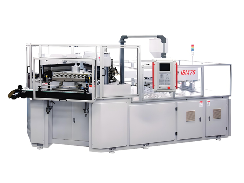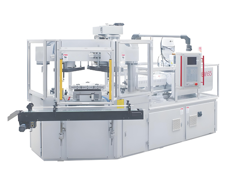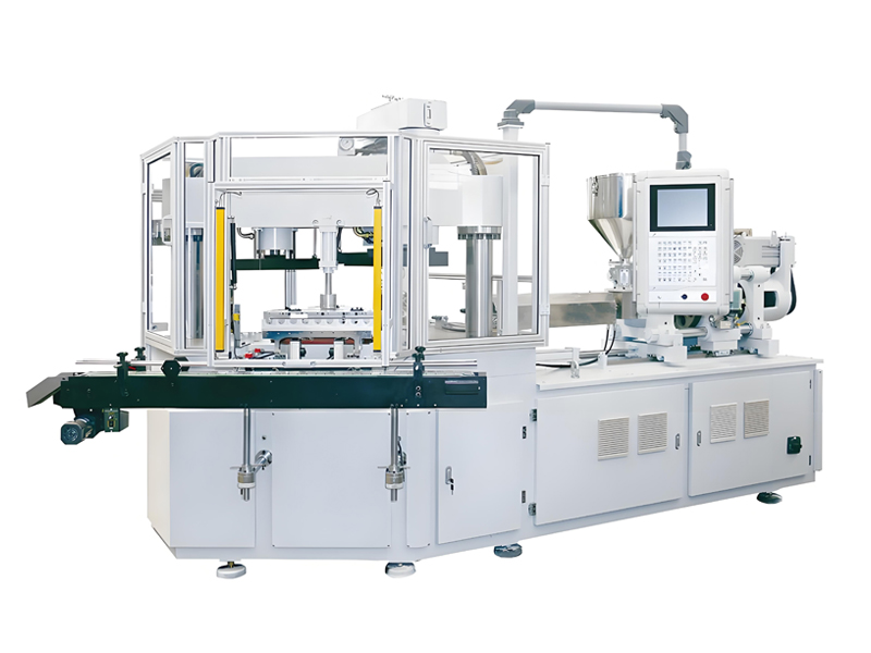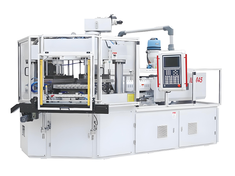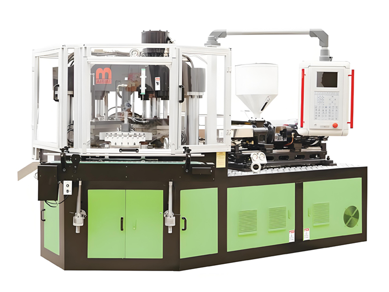
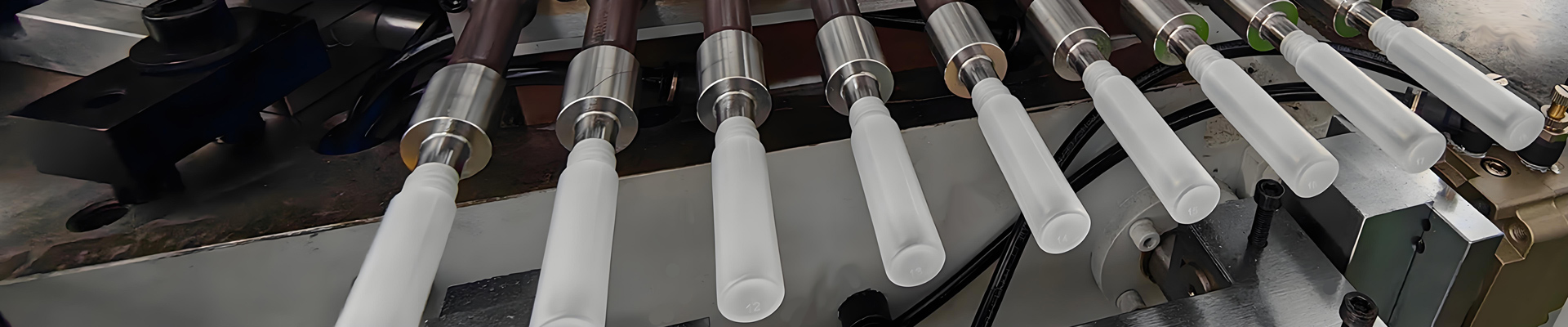
Aibim, a Wanplas factory, builds three-station one-step injection blow molding (IBM) machines for precise small containers used in pharmaceuticals, cosmetics, food and daily chemicals. The IBM55 Hybrid, IBM65 and IBM75 produce bottles from 3 ml to 1000 ml in PE, PP, PS, ABS, SAN, TPU, PC and PCTG. In this process the plasticizing barrel, the hot runner or manifold, the nozzle and the blow mold must each sit at a deliberately different temperature, and those temperatures must hold steady across millions of cycles. A Gefran multi-zone temperature controller is the instrument that delivers that stability. This article explains the architecture of precision heating control on an IBM machine, the sensors and outputs involved, the protection features that prevent scrap and fire risk, and the direct line between a well-shaped temperature curve and the quality of the finished bottle. The discussion is relevant whether the controller is supplied as a standalone rack or integrated into the machine’s higher-level Siemens control system.

Why Heating Precision Defines IBM Quality

Injection blow molding begins by melting resin in an injection barrel and forming a parison or preform on a core rod. If the melt is too cold, the parison fills unevenly and the bottle shows short shots or weak corners. If the melt is too hot, the resin degrades, the neck finish loses definition and the bottle may pick up color change or odor that fails pharmaceutical and cosmetic specifications. Between those extremes, small swings of a degree or two shift the viscosity enough to change wall thickness distribution, especially in thin-walled cosmetic jars where the tolerance is tight.

The control problem is harder than it looks because heating is slow and lagging while cooling is fast. A barrel zone heated by a band at a few W/cm2 takes time to reach temperature, but once energized it overshoots if the controller is naive. A Gefran loop using tuned PID and sometimes fuzzy logic anticipates that lag, brakes the overshoot and settles the zone within a narrow band. That stability is what lets an Aibim machine hold the claimed minimum 35 percent energy saving, because energy is not wasted fighting oscillation or reheating after a drift.

Heating precision also protects the asset. Over-temperature events stress heater bands, degrade insulation and can char residual material in dead spots. A controller with proper alarm and protection logic turns a potential burnout into a logged warning and a controlled shutdown, extending the life of bands and thermocouples alike.

Multi-Zone Temperature Control Architecture

An IBM machine is not heated as one block. It is divided into functional zones, each with its own sensor, controller channel and power stage. A typical Aibim IBM75 might carry more than a dozen zones: rear, middle and front barrel zones, an adapter or manifold zone, a nozzle zone, and several blow-mold cooling or conditioning zones where the story is really about holding a low, stable mold temperature rather than heating.

The Gefran architecture groups these channels in a compact format, often with one controller module handling several loops and sharing a communication bus back to the main PLC. Each loop is independent: the rear barrel can sit near 200 deg C for PP while the front zone runs higher to ensure melt homogeneity, and the mold can be held near shop-cooling temperature by a separate conditioning circuit. Independence matters because coupling zones through a single setpoint would force a compromise that hurts either plasticizing or product surface.

Zone	Typical role	Control objective
Rear barrel	Feed, gentle preheat	Stable feed, no bridging
Middle barrel	Main plasticizing	Homogeneous melt
Front barrel	Final melt conditioning	Viscosity for fill
Manifold / hot runner	Parison transfer heat	No freeze, no degradation
Nozzle	Gate and injection point	Clean shutoff, no drool
Blow mold	Cooling / conditioning	Dimensional stability

Thermal coupling between adjacent zones

Independence at the controller level does not mean independence in the steel. Barrel zones are bolted to one continuous cylinder, so heat conducts axially between them. A zone that is driven hard will export perhaps 3 deg C to 8 deg C into its neighbour within two or three minutes, and the neighbouring loop sees that as an unexplained rise it must reject with reduced output. On a 12-zone IBM75 this cross-talk is the single most common reason a freshly commissioned machine shows a slow, wandering profile even though every individual loop was autotuned correctly.

Three practical countermeasures apply. First, stage the setpoints so the gradient between adjacent barrel zones stays modest, ideally no more than 15 deg C to 25 deg C per zone step, which keeps the conducted flux small relative to each zone’s own heater capacity. Second, give the downstream zone a slightly longer integral time, typically 20 percent to 40 percent longer than the upstream zone, so it absorbs rather than fights the imported heat. Third, respect the mechanical breaks: the adapter flange between barrel and manifold and the insulating plate under the nozzle are deliberate thermal resistances, and removing an insulating washer during a rebuild can silently couple two zones that were designed to be separated.

Hot runner and manifold zones behave differently again. A manifold is a hot mass surrounded by a relatively cool mold plate, so its dominant disturbance is not the neighbouring zone but the heat sink of the tool itself. When the mold opens and closes, and when cooling water flows through the plate at 10 deg C to 20 deg C, the manifold loses energy in a rhythm locked to the cycle. A well-configured Gefran loop with a derivative term sized to the cycle period rides that rhythm instead of chasing it, keeping the manifold within a few tenths of a degree cycle-to-cycle.

The blow mold conditioning zones invert the logic once more. Here the controller is usually modulating a cooling circuit or a small trim heater to hold a target such as 12 deg C to 30 deg C depending on resin. Coupling runs from the hot core rod into the cold cavity every cycle, so the mold zone experiences a periodic heat pulse whose amplitude scales with shot weight. When a customer changes from a 10 ml vial to a 500 ml bottle on the same tool family, the mold loop often needs a fresh tune even though nothing electrical has changed.

For comparison, competing IBM builders such as Jomar and Milacron use comparable multi-zone layouts, and the underlying control principles are the same even when the brand of controller differs. What distinguishes a well-executed Aibim cell is the combination of zone count, sensor placement close to the process, and tight integration with the Siemens supervisor so that a temperature deviation is not just displayed but acted upon.

PID Autotuning and Fuzzy Control

The proportional-integral-derivative (PID) algorithm is the workhorse of temperature control. The proportional term reacts to the current error, the integral term removes steady offset, and the derivative term anticipates trend to damp overshoot. A poorly tuned PID either oscillates or responds sluggishly; a well-tuned one settles quickly and holds.

Gefran controllers offer PID autotuning, where the instrument performs a controlled excitation of the zone, observes the thermal response, and calculates suitable P, I and D values automatically. This saves the technician from manual trial-and-error and gives a repeatable starting point across identical machines. On an Aibim line where several IBM65 units run the same product, autotuning each to the same baseline keeps their output consistent.

Fuzzy control is the complementary technique. Where classical PID needs a precise mathematical model, fuzzy logic uses linguistic rules such as “if error is small and rising fast, reduce power moderately.” This handles the non-linear behavior of heating elements whose response changes as bands age or as ambient conditions shift. Many modern controllers blend PID with fuzzy adaptation so that the loop self-adjusts as the heater band’s characteristics drift over months of service.

Approach	Strength	Best use on IBM
Manual PID	Full technician control	Rare, bespoke tuning
PID autotune	Fast, repeatable setup	Commissioning, fleet consistency
Fuzzy adaptive	Handles non-linear drift	Aged bands, ambient swings
PID + fuzzy blend	Stable and self-correcting	Long-term production

When autotuning fails and how to recognise it

Autotuning is not infallible. It assumes the zone is thermally quiet during the test, that the heater has enough headroom to excite a clear response, and that the sensor is reading the same mass the heater is warming. Break any of those assumptions and the calculated parameters will be wrong in a way that is not obvious until production starts. The typical symptoms are recognisable once you know them.

• Sustained oscillation of 2 deg C to 6 deg C peak to peak with a regular period: proportional band too narrow or derivative time too short. The loop is over-reacting to its own corrections.
• Large first overshoot of 10 deg C to 25 deg C followed by a slow settle: integral action too aggressive during the warm-up ramp, a classic result of autotuning a zone that was already partly warm.
• Permanent offset of 1 deg C to 3 deg C that never closes: integral time far too long, or the output is clamped by a power limit the technician forgot was active.
• Very slow approach taking more than 25 minutes for a barrel zone that should reach setpoint in 8 minutes to 15 minutes: proportional band too wide, or the heater band has lost contact with the barrel and the real thermal path is worse than the tune assumed.
• Autotune aborts and reverts to defaults: usually a sensor fault, an interlock removing power mid-test, or an ambient draught from an open guard door.

The correct response to a failed autotune is to fix the physical cause and retry from a genuinely cold, stable start, not to run the tune repeatedly and hope. If the zone still refuses to tune, manual tuning is straightforward using the classical Ziegler-Nichols closed-loop method. Set integral and derivative off, raise the proportional gain until the zone oscillates with a constant amplitude, record that ultimate gain Ku and the oscillation period Tu in seconds, then read the parameters from the table below.

Controller mode	Proportional gain Kp	Integral time Ti	Derivative time Td
P only	0.50 Ku	Not used	Not used
PI	0.45 Ku	0.83 Tu	Not used
Classic PID	0.60 Ku	0.50 Tu	0.125 Tu
Low-overshoot PID	0.33 Ku	0.50 Tu	0.33 Tu
No-overshoot PID	0.20 Ku	0.50 Tu	0.33 Tu

For heat-only plastics zones the low-overshoot or no-overshoot rows are usually the right starting point, because an overshoot of even 15 deg C on a heat-sensitive resin such as PVC-adjacent compounds or a filled PP can leave degraded material sitting in the flow path. Note that most Gefran and comparable instruments express proportional action as a proportional band in degrees rather than a dimensionless gain; the band in degrees is simply the span divided by the gain, so a Kp of 4 on a 400 deg C span corresponds to a band of 100 deg C. Confirm which convention the instrument uses before entering numbers, since entering a gain where a band is expected produces an almost comically sluggish loop.

Fuzzy adaptation sits on top of whichever base tune you arrive at. Rather than recomputing P, I and D, it applies a correction to the output based on the error magnitude and the rate of change, using a rule set that is tolerant of an imperfect model. In practice this means the loop that was tuned in a 22 deg C workshop in winter still behaves acceptably at 34 deg C in summer, and the loop tuned on a new heater band does not need retuning when that band’s resistance has crept up by 5 percent to 8 percent after 8000 hours of service.

The practical payoff is reduced operator intervention. Once autotuned and adapted, the loops hold setpoint with minimal attention, and the technician’s time shifts from firefighting temperature to optimizing the rest of the cycle.

Thermocouple J/K and Pt100 Accuracy

A controller is only as good as its measurement. The sensor converts temperature into a signal the controller compares against setpoint. Two common choices appear on IBM machines: thermocouples, especially type J and type K, and resistance thermometers such as Pt100.

Type J thermocouples use iron-constantan and suit moderate temperature ranges typical of barrel heating, while type K (chromel-alumel) offers a wider range and better oxidation resistance, making it common near nozzles and manifolds. Thermocouples are robust and cheap but have lower absolute accuracy and are sensitive to electrical noise and lead-length effects. Pt100 is a platinum resistance sensor with high accuracy and stability, often used where the spec calls for tight control, such as mold conditioning or validation points that feed the batch record.

Sensor	Typical range	Accuracy class	IBM use
Type J TC	Around -40 to 750 deg C	Moderate	Barrel, general zones
Type K TC	Around -200 to 1300 deg C	Moderate	Nozzle, manifold
Pt100	Around -200 to 600 deg C	High, stable	Mold, validation points

Accuracy classes and cold-junction compensation

Sensor accuracy is defined by tolerance class rather than by a single number. A class 2 thermocouple is typically specified at the greater of 2.5 deg C or 0.0075 times the absolute reading, which at a barrel setpoint of 230 deg C means a permissible error of about 2.5 deg C. A class 1 thermocouple tightens that to the greater of 1.5 deg C or 0.004 times the reading, roughly 1.5 deg C at the same point. A Pt100 to class A is specified at about 0.15 deg C plus 0.002 times the temperature, giving roughly 0.6 deg C at 230 deg C, and a class AA or 1/3 DIN element halves that again. This is why validation points and mold conditioning circuits favour Pt100 while general barrel zones are perfectly served by a class 2 type J.

Whatever the class, a thermocouple only produces a voltage proportional to the difference between the hot junction and the terminal block where it lands. The controller must therefore measure its own terminal temperature and add the corresponding offset, which is cold-junction compensation. Two conditions break it. The first is using ordinary copper wire instead of matched compensating cable, which relocates the effective cold junction to an unmeasured point in the cabinet. The second is a hot terminal strip: a cabinet running at 55 deg C when the controller’s internal reference assumes a gentler rise will bias every zone by 1 deg C to 3 deg C in the same direction, a fault that looks like a calibration drift affecting the whole machine at once.

Shielding, grounding and polarity

A thermocouple signal is only 40 microvolts to 55 microvolts per degree for type K and about 50 microvolts to 60 microvolts per degree for type J. That is a tiny signal running through a cabinet containing thyristor stacks, servo drives and contactors, so noise rejection is not optional. Use twisted-pair compensating cable with an overall foil or braid screen, keep the run physically separated from power cabling by at least 100 mm to 200 mm, and cross power cables at right angles where separation is impossible. Ground the screen at one end only, normally the cabinet end, because grounding both ends invites a circulating current in the screen that couples straight back into the pair.

Grounded-tip versus ungrounded-tip probes is a related decision. A grounded tip responds faster, often 1 second to 3 seconds quicker on a barrel probe, but it ties the measuring circuit to machine earth and can create a ground loop if the controller input is not isolated. An ungrounded tip is slower but electrically clean and is the safer default on a machine with phase-angle thyristors, which inject significant switching noise. Where a grounded tip is unavoidable, an isolated input module is worth the modest extra cost.

Reversed polarity is the classic wiring error and it has a distinctive signature. Because the instrument still applies cold-junction compensation correctly but the measured thermoelectric voltage now has the wrong sign, the display falls as the zone heats up. A zone that reads 18 deg C when the cabinet is at 25 deg C, then drifts down towards 10 deg C as the band warms, is almost certainly reversed. Type J is white for negative and black for positive under the common colour convention, type K is red for negative and green or yellow for positive depending on the standard applied, and the reliable field test is simply that the negative leg of both J and K is magnetic on the iron and alumel conductors respectively. A quick check with a small magnet at the terminal saves an hour of chasing a phantom controller fault.

Two further sensor faults deserve a mention. A partially broken thermocouple produces an intermittent, jumpy reading rather than a clean open circuit, typically flicking 5 deg C to 40 deg C at random intervals; the controller sees this as violent error and modulates power erratically. And a Pt100 wired as two-wire rather than three-wire adds the lead resistance directly to the measurement, roughly 0.4 deg C per ohm of loop resistance, so a long two-wire run can read several degrees high with no other symptom.

Sensor placement is as important as sensor type. A thermocouple buried deep in the barrel wall reads the metal, not the melt; a sensor in a well touching the melt path reads process temperature but is harder to fit. Aibim positions sensors to reflect the zone that actually drives quality, and the controller is configured with the correct input type and cold-junction compensation so the displayed value matches reality. Periodic calibration against a reference keeps the audit trail credible for ISO 15378 and GMP contexts.

SSR and Thyristor Power Output

The controller decides a temperature, but a power stage delivers energy to the heater band. Two common output technologies are the solid-state relay (SSR) and the thyristor (silicon-controlled rectifier) module.

An SSR switches the load fully on or off, typically once per mains half-cycle or via zero-cross switching. It is simple, cheap and reliable for lower-power zones, but because it is effectively bang-bang at the switching boundary, fine control relies on the controller’s time-proportioning. A thyristor, by contrast, can phase-angle fire, delivering a variable fraction of each half-cycle to the load. This gives much smoother power delivery, less thermal cycling of the band, quieter operation and finer regulation, which is valuable on high-power barrel zones where hunt and overshoot waste energy and stress the element.

Output type	Control style	Relative cost	IBM fit
SSR, zero-cross	On/off proportioning	Low to Medium	Lower-power zones
Thyristor, phase-angle	Continuous modulation	Medium to High	High-power barrel zones
Thyristor, burst-fire	Cycle proportioning	Medium	Medium zones, less EMI

Zero-cross firing versus phase-angle firing

The distinction that matters electrically is when in the mains waveform the device turns on. Zero-cross, also called burst-fire, waits for the voltage to pass through zero before conducting and then passes whole half-cycles. On a 50 Hz supply each half-cycle is 10 ms, so the smallest quantum of energy the stage can deliver is one 10 ms slice. Over a proportioning cycle of 1 second to 2 seconds that gives resolution of roughly 0.5 percent to 1 percent of full power, which is ample for most zones. Because switching happens at zero volts, the generated electromagnetic interference is very low and the stage is friendly to nearby analogue signals.

Phase-angle firing turns the device on partway through each half-cycle, chopping the waveform to deliver anything from a few percent to full power with effectively continuous resolution. The advantage on a 6 kW to 12 kW barrel zone is real: power flows every half-cycle instead of arriving in bursts, the band’s own surface temperature ripple falls from perhaps 8 deg C to 15 deg C down to 1 deg C to 3 deg C, and element fatigue from repeated expansion and contraction drops accordingly. The disadvantage is the abrupt current step at the firing point, which generates conducted and radiated interference and injects harmonic currents into the supply.

Characteristic	Zero-cross / burst	Phase-angle
Smallest energy step	One 10 ms half-cycle	Continuous within each half-cycle
Conducted interference	Very low	Significant, needs filtering
Harmonic content	Low order, mild	Rich, 3rd and 5th prominent
Supply flicker risk	Possible on weak supply	Low, load is smooth
Band thermal ripple	Around 8 to 15 deg C	Around 1 to 3 deg C
Relative cost	Low to Medium	Medium to High

Neither is universally correct. On a site with a stiff supply and short cable runs, burst-fire on every zone is a perfectly sound Low cost choice and the flicker it causes is invisible. On a site where several IBM machines share a transformer with lighting and inspection cameras, the repeated stepping of 40 A to 60 A blocks of load can produce visible flicker and can upset sensitive instruments, and phase-angle with an input filter is the better engineering answer despite the Higher cost. A useful hybrid, and the arrangement Aibim commonly specifies, is phase-angle on the two or three dominant barrel zones and burst-fire on the low-power nozzle and auxiliary loops, which captures most of the control benefit at a Medium overall cost.

Harmonic mitigation deserves a sentence of its own. Phase-angle stages draw non-sinusoidal current, and the resulting third and fifth harmonics circulate in the neutral of a three-phase system. Balancing heater loads across the three phases at commissioning, so that no phase carries more than about 10 percent more current than the others, is the cheapest and most effective mitigation. Where a facility already runs close to its harmonic limits, delay-triggered soft-start on the thyristor stack and a line reactor of 2 percent to 4 percent impedance will usually bring distortion back inside the site specification without further investment.

Selection balances control quality against budget. Aibim’s energy-saving design benefits most from thyristor control on the dominant barrel zones, while SSRs can serve auxiliary or low-power loops at a lower relative cost. Competing controller brands such as Eurotherm and Watlow offer equivalent thyristor stages, but the integration and zone mapping matter more than the badge on the module.

Soft Start, Power Limiting and Load Monitoring

When a cold IBM machine is powered up, every heater band is at ambient and draws full current until it warms. A soft start limits the initial power ramp so the incoming supply is not stressed and the bands are not thermally shocked. This prolongs element life and avoids tripping the workshop breaker on a Monday-morning start across multiple machines.

Power limiting caps the total energy a zone or the whole rack may draw, useful when the site has a constrained electrical supply or when running several IBM75 lines on one feeder. Load monitoring goes further: the controller measures the current or resistance of each band and compares it to the expected value. A band that has partially failed draws abnormal current; the system flags it before it fails completely and causes a temperature sag that quietly degrades bottle quality.

A drifting heater band is the silent killer of IBM consistency. Load monitoring turns that silent failure into a scheduled maintenance task rather than a mystery scrap run.

These features also support energy accounting. By knowing each zone’s kWh and comparing it to a baseline, a plant can spot a band losing efficiency or a setpoint left too high, then correct it. Within the Aibim value story of lower energy consumption, disciplined power limiting and monitoring are concrete ways the saving is achieved and sustained rather than claimed once at commissioning.

Break-Thermocouple Protection and Overtemp Alarm

Two failure modes dominate temperature safety. The first is a broken thermocouple. If the sensor opens, a naive controller may read a very low temperature and drive the band to full power forever, scorching the barrel and the resin. Break-thermocouple protection detects the open circuit and either holds the output at a safe value or shuts the zone down, logging the fault.

The second is over-temperature. Even with good control, a stuck SSR or a failed band can push a zone past its limit. The controller’s overtemp alarm compares the measured value against a configurable ceiling and triggers a warning or interlock. On regulated lines this alarm is also forwarded to the higher-level Siemens PLC and recorded, so the event becomes part of the traceability record rather than a silent trip.

Protection	Trigger	Controller response
Break-thermocouple	Open sensor circuit	Safe hold or shutdown, log
Overtemp alarm	Measured above ceiling	Warn, interlock, forward to PLC
Deviation alarm	Setpoint gap too wide	Operator alert, possible hold
Heater fault	Abnormal load current	Maintenance flag

Aibim machines carry CE certification and integrate safety states through the control system, so a temperature fault is not an isolated instrument beep but a coordinated response that protects the operator, the mold and the batch. For pharmaceutical customers this coordination is part of what makes the line acceptable during qualification.

Heater Band Power Density and Zone Layout

Heater band power density, expressed in watts per square centimeter (W/cm2), describes how concentrated the heating power is on the barrel surface. A higher density band reaches temperature faster and fits in a compact space, but it runs hotter locally and can create hot spots if not matched to the zone. A lower density band spreads heat more gently and is kinder to sensitive resins, at the cost of slower response and more physical length.

Correct zone layout matches band density to the thermal duty. The rear feed zone needs gentle, lower-density heating to avoid melting too early and bridging; the front and manifold zones may use higher density to condition the melt quickly. The blow mold is a different story: it is usually cooled, not heated, and its “control” is about holding a stable low temperature through a conditioning circuit rather than applying W/cm2.

Zone	Typical band density	Design intent
Rear barrel	Lower density	Avoid early melt, bridging
Middle barrel	Medium density	Steady plasticizing
Front / manifold	Higher density	Fast melt conditioning
Nozzle	Medium to high	Localized, stable gate

Band construction, W/cm2 rating and service life

Density alone does not describe a band. Construction determines the maximum surface temperature the element can survive, how well it tolerates contamination from purged resin, and how long it lasts. The four families found on IBM machines differ substantially.

Band type	Typical density	Max sheath temp	Indicative life	Relative cost
Mica insulated	2.5 to 4.5 W/cm2	Around 480 deg C	8000 to 15000 h	Low
Ceramic knuckle	4.0 to 7.5 W/cm2	Around 700 deg C	15000 to 30000 h	Medium
Cast aluminium / bronze	2.0 to 4.0 W/cm2	Around 400 deg C	25000 to 40000 h	High
Ceramic infrared	3.0 to 6.0 W/cm2	Around 750 deg C	10000 to 20000 h	Medium to High

Reading the table against the IBM duty cycle gives clear guidance. Mica bands are the Low cost workhorse for rear and middle barrel zones on commodity PE and PP, where the required surface temperature is modest and a band change every two to three years is acceptable. Ceramic knuckle bands earn their Medium cost on front barrel and manifold zones because the air gap in their construction tolerates the higher sheath temperature and the thermal cycling of a hot runner. Cast aluminium bands are the Premium option for zones where uniformity is paramount and where a purge of hot resin would destroy a mica band; the cast body distributes heat so evenly that cross-band spread often falls below 5 deg C, and because the element is embedded the life is the longest of the four. Infrared elements appear on specialised preform conditioning rather than on the barrel itself.

A practical rule for sizing is to calculate the required power from the barrel mass and the target warm-up time, then choose the lowest density that meets it. A 90 mm barrel section 200 mm long has roughly 565 cm2 of surface; at 3.5 W/cm2 that is about 1.98 kW, comfortably enough to raise that section to 230 deg C in 12 minutes to 18 minutes from cold. Pushing the same section to 6 W/cm2 would reach setpoint faster but the sheath would run 60 deg C to 100 deg C hotter for the same delivered energy, which is exactly the condition that shortens life and creates local hot spots the sensor never sees.

Fit is the other half of life expectancy. A band that has lost intimate contact with the barrel, whether because the clamp has relaxed or because carbonised resin has built up underneath, transfers heat far less efficiently, so the element runs hotter to achieve the same barrel temperature. A gap of only 0.2 mm can raise element temperature by 40 deg C to 80 deg C and cut life by half or more. Re-torquing barrel clamps at each planned maintenance, and cleaning the barrel surface whenever a band is removed, is a few minutes of work that repays itself many times.

The controller must know the band it drives. A zone tuned for a high-density band will behave differently with a low-density replacement, so Aibim’s commissioning records the band specification per zone and the controller parameters are set accordingly. When a band is replaced in the field, matching density and re-confirming the loop keeps quality stable instead of introducing a subtle shift the operator cannot see.

Temperature Uniformity Across the Profile

Uniformity has two meanings on an IBM line. Within a single zone, it is how tightly the controller holds the setpoint, typically expressed as plus or minus a fraction of a degree under steady load. Across the machine, it is how evenly the intended profile is realized along the barrel and through the manifold, which depends on band placement, density, sensor location and the mechanical contact between band and steel.

A well-tuned Gefran multi-zone loop commonly holds a stable zone within roughly plus or minus 0.5 deg C of setpoint under steady conditions, while the cross-manifold uniformity depends more on mechanical design than on the controller alone. Both matter: tight within-zone control prevents oscillation, and good cross-zone uniformity prevents one section from being hotter than the resin can tolerate.

Metric	Typical target	Main influence
Within-zone stability	Around plus or minus 0.5 deg C	Loop tuning, output type
Cross-manifold spread	Few deg C by design	Band layout, contact
Setpoint tracking	Minimal offset	Integral action, autotune

What a half-degree actually buys

It is easy to treat plus or minus 0.5 deg C as a marketing figure. It is not. The viscosity of a semi-crystalline polyolefin melt changes by roughly 2 percent to 4 percent per degree in the normal processing window, and for an amorphous resin such as PC or PCTG the sensitivity can reach 5 percent to 8 percent per degree near the lower end of the window. A loop wandering plus or minus 3 deg C therefore presents the injection unit with a melt whose flow resistance varies by 10 percent or more shot to shot, and a constant injection profile will fill that parison differently each time.

The downstream consequences are measurable on four separate quality attributes.

• Wall thickness distribution. On a 250 ml PE bottle with a nominal 0.55 mm sidewall, a plus or minus 0.5 deg C loop typically keeps thickness variation inside about 0.03 mm, while a plus or minus 3 deg C loop widens that to 0.08 mm to 0.12 mm. Since drop-test performance and top-load strength are governed by the thinnest point, the wider distribution forces the process engineer to add material everywhere to protect the worst case, raising part weight by 3 percent to 6 percent.
• Transparency and gloss. Clarity in PCTG, SAN and PC bottles depends on avoiding both under-melted gel particles and thermally degraded micro-yellowing. Both failure modes sit at opposite ends of the temperature band, so the usable window may be only 12 deg C to 20 deg C wide. A loop that consumes 6 deg C of that window in oscillation leaves very little margin for resin lot variation.
• Residual stress. Uneven cooling and inconsistent melt temperature freeze differential stress into the sidewall and, more critically, into the neck and the transition radius. Stress shows up later as environmental stress cracking with aggressive cosmetic formulations, or as dimensional creep that causes cap torque to fall below specification after several weeks in a warehouse at 40 deg C.
• Neck finish and seal integrity. The thread and sealing surface are formed by the injection stage, not the blow stage, so they inherit melt temperature stability directly. A drifting nozzle zone produces flash on one shot and an incompletely packed thread on the next, and for pharmaceutical closures that is a container-closure integrity risk rather than a cosmetic one.

Cross-zone uniformity has a parallel effect. If a four-cavity manifold shows an 8 deg C spread between the hottest and coolest drop, the four bottles will differ systematically in weight by 1 percent to 2 percent and in wall distribution by more, and no amount of loop tuning will fix it because each drop is individually stable at the wrong temperature. That is a mechanical and heater-layout problem, diagnosed by mapping the drops with a calibrated reference probe during a warm hold and corrected by rebalancing band power or adding insulation where the manifold contacts the plate.

Uniformity is also a validation parameter. On pharmaceutical lines the documented temperature performance supports the equipment qualification record, and a controller that logs actual zone temperatures gives the evidence that the machine ran within the validated window during a batch.

Modbus RTU and Fieldbus Communication

A temperature controller rarely works alone. It communicates with the machine’s main control system so that setpoints, actual values and alarms flow both ways. Modbus RTU is a widely used serial protocol over RS-485 that lets the Gefran rack exchange data with a Siemens PLC or a supervisory computer. It is simple, robust and supported by almost every industrial device, which is why it remains common even as faster fieldbuses spread.

Beyond Modbus RTU, modern controllers support fieldbus options that place the temperature loops directly on the machine network, reducing wiring and giving the supervisor richer, faster data. The choice depends on the architecture: a retrofit may use Modbus RTU because the existing PLC already polls it, while a new IBM75 built around PROFINET may prefer a fieldbus node so temperature becomes just another set of tags in the S7-1500 project.

Bus	Physical	IBM use
Modbus RTU	RS-485 serial	Retrofit, simple polling
PROFINET	Industrial Ethernet	New S7-1500 integration
Other fieldbus	Vendor specific	Mixed-vendor cells

Register mapping and PLC integration in practice

Configuring the link is mostly a matter of agreeing the serial parameters and the register map. A typical Gefran rack on RS-485 runs at 9600 baud or 19200 baud, 8 data bits, no parity or even parity, 1 stop bit, with each controller assigned a unique slave address from 1 to 247. Termination resistors of 120 ohm belong at the two physical ends of the bus and nowhere else, and the total run should stay under about 1200 m at the lower baud rate. A missing termination shows up as intermittent CRC errors that the PLC logs as occasional timeouts rather than as an outright failure, which makes it one of the more irritating commissioning faults to trace.

The register map itself follows a predictable pattern. Process value, setpoint, output percentage, alarm status word and the PID parameter block each occupy defined holding registers, usually as 16-bit integers scaled by ten so that 2305 represents 230.5 deg C. The PLC reads the process values and status words continuously, typically on a 200 ms to 1000 ms poll, and writes setpoints only on change. Writing setpoints every scan is a common integration mistake: many instruments store setpoints in non-volatile memory with a finite write endurance, and hammering that register can wear it out within a year.

Data item	Direction	Typical scaling	Suggested poll rate
Process value per zone	Read	0.1 deg C per count	200 to 500 ms
Setpoint per zone	Read and write	0.1 deg C per count	On change only
Output power percent	Read	0.1 percent per count	500 to 1000 ms
Alarm and status word	Read	Bit-mapped	200 ms
Load current per zone	Read	0.1 A per count	1 to 5 s
PID parameter block	Read and write	Instrument specific	On recipe change

Once the tags exist in the S7-1500 project they can be used for far more than display. Recipe management writes the whole setpoint set for a given resin and bottle in one operation, eliminating the transcription errors that come from an operator typing eleven numbers into a keypad. A start interlock can prevent the injection unit from moving until every zone is within 3 deg C of setpoint and has been stable for a defined soak of 10 minutes to 20 minutes, which protects the screw and eliminates the first-shots-are-scrap habit. And a deviation from setpoint can be latched against the production batch record rather than merely flashing on a panel.

Temperature trend archiving closes the loop on traceability. Logging every zone at 1 s to 5 s intervals for the duration of a batch produces a modest data volume, on the order of a few megabytes per shift for a 12-zone machine, and gives quality assurance the ability to answer the awkward question of what the machine was doing at the moment a suspect bottle was produced. Where a customer works to 21 CFR Part 11 expectations, the archive needs time stamping, user attribution for setpoint changes and protection against alteration, all of which are functions of the SCADA layer rather than the temperature controller itself, but which depend entirely on the controller exposing the data reliably in the first place.

Communication also enables remote support. With the temperature data on the network, an Aibim engineer can review zone trends from the China headquarters, much like the remote-monitoring philosophy the Wanplas group applies across its factories, shortening the gap between a drifting zone and a corrected setpoint.

How the Temperature Curve Shapes Melt and Product

Everything above serves one purpose: the right temperature curve through the machine. The curve is the set of zone temperatures along the melt path, and small changes reshape the bottle. For PP in a pharmaceutical bottle, a slightly higher melt temperature improves flow and neck definition but raises the risk of odor and warp if pushed too far. For PETG in a cosmetic jar, the window is narrower and stray heat dulls clarity.

The practical link is viscosity. Temperature sets melt viscosity, viscosity sets how the parison forms and how it inflates against the blow mold, and that sets wall thickness distribution. A stable controller keeps viscosity stable, so the wall thickness measured by quality stays inside tolerance and the rejection rate stays Low. An unstable controller lets viscosity wander, producing intermittent thin spots that pass one hour and fail the next.

Temperature effect	If too low	If too high
Barrel melt temp	Short shot, weak corners	Degradation, odor, warp
Manifold temp	Freeze, flow marks	Drool, degradation
Mold temp	Slow cycle, stress	Sticking, dimensional drift
Stability (all zones)	Thick/thin variation	Same, unpredictable

The conclusion for a buyer is that temperature control is a quality system, not a comfort setting. Specifying Gefran multi-zone controllers with autotuning, accurate Pt100 or type J/K sensing, thyristor output on power zones, and full alarm and communication integration gives an Aibim IBM machine the thermal stability that the bottle quality, the energy bill and the audit record all depend on. Wanplas, the parent brand, reinforces this with shared quality standards and an open-factory policy so customers can verify the engineering before they commit.

Thermal Runaway and Layered Safety Interlocks

Break-thermocouple detection and an overtemperature alarm are the first two layers of protection, but they do not cover every path to a runaway. Thermal runaway on an IBM machine means a zone continues to gain energy after the control system has decided it should stop. The three mechanisms that cause it are a welded or shorted output device, a control loop that is heating a different mass from the one it is measuring, and an operator or recipe error that sets a ceiling above what the material can survive.

A shorted SSR is the most common. Solid-state devices usually fail closed rather than open, so a stack that fails at 06:00 will simply pour full power into its band until something else notices. The controller sees the temperature climbing while its own output demand sits at zero percent, and that specific combination is the diagnostic signature. A well-configured instrument raises a heater-short alarm on exactly that logic within 30 s to 90 s.

Building the protection in layers

Because no single detector is trustworthy on its own, protection is layered so that each layer covers the previous layer’s blind spot.

Layer	Mechanism	Typical trip setting	Action
1. Deviation alarm	Software, same loop	Setpoint plus 8 to 15 deg C	Warn operator, log
2. Absolute high alarm	Software, fixed ceiling	Setpoint plus 25 to 40 deg C	Inhibit injection, hold cycle
3. Heater-short detection	Current sensed at zero demand	Above 5 percent of rated A	Drop zone contactor
4. Group safety contactor	Hardwired, PLC driven	Any layer 3 event	Remove power from all bands
5. Independent thermostat	Electromechanical, separate sensor	Around 60 deg C above max process	Break control circuit directly

The essential feature of layer 4 and layer 5 is independence. The group contactor must be driven by a circuit that does not depend on the same output device that failed, and the layer 5 thermostat must use its own sensing element wired directly into the control circuit so that it functions even if the controller, the PLC and the network are all dead. This is the difference between a machine that logs a fault and a machine that starts a fire, and it is a large part of what a CE assessment examines when it looks at heating circuits.

Two operational practices reinforce the hardware. The first is a maximum-setpoint clamp configured per zone, so that even a mistyped recipe cannot ask for 320 deg C on a zone that should never exceed 260 deg C. The second is a soak interlock on restart after any thermal fault: the machine should require a deliberate acknowledgement and a fresh warm-up rather than resuming automatically, because a zone that tripped once will usually trip again and each unattended cycle bakes the resin sitting in the flow path a little further.

Protection that shares a component with the thing it protects against is not protection. Every layer must be able to act when the layer above it has already failed.

Finally, the melt itself deserves consideration. Most engineering resins begin to release decomposition products well before they visibly char, and some grades generate significant pressure inside a blocked nozzle. A runaway that is caught at 40 deg C above setpoint is a cleaning job; one caught at 150 deg C above setpoint can be a purge hazard requiring the barrel to be cooled and cleared under controlled conditions. Setting layer 2 conservatively costs nothing in production terms because a healthy machine never approaches it.

Calibration, Verification and Traceability Records

A controller displaying 230.0 deg C is making a claim, and in a regulated packaging environment that claim has to be defensible. Calibration is the process of comparing the whole measurement chain against a reference of known accuracy and either adjusting it or recording the deviation. Verification is the lighter-weight periodic check that confirms the chain has not drifted since the last calibration.

What actually drifts

The controller’s own analogue front end is usually the most stable element, typically drifting less than 0.1 deg C per year. The sensor is the weak link. A type J thermocouple exposed to 250 deg C continuously will drift by 1 deg C to 3 deg C over 12000 hours to 20000 hours as the iron leg oxidises and the alloy composition at the junction changes, and the drift is almost always in one direction so it accumulates rather than averaging out. Pt100 elements are far more stable, often within 0.1 deg C over several years, but they are vulnerable to mechanical shock and to moisture ingress at the head, both of which produce a step change rather than a slow drift.

Activity	Suggested interval	Acceptance criterion	Record produced
Controller input simulation check	12 months	Within 0.5 deg C at three points	Calibration certificate
Loop verification with reference probe	6 months	Within 2 deg C of reference	Verification log entry
Barrel thermocouple replacement	24 to 36 months	On drift or on schedule	Maintenance record
Reference instrument recertification	12 months	Traceable to national standard	Accredited certificate
Alarm and interlock function test	6 to 12 months	All layers trip as designed	Safety test report

Note the distinction between the first two rows. Simulating a thermocouple input at the controller terminals tests the instrument but says nothing about the sensor in the barrel. Verifying the loop with an independent reference probe inserted into the same well tests the whole chain but is harder to arrange and cannot easily be done at more than one temperature. A sound programme uses both: an annual instrument calibration that produces a certificate, and a six-monthly loop check that catches sensor drift between certificates.

Documentation expectations in GMP and ISO 15378 contexts

Customers producing primary packaging for medicinal products work to ISO 15378, which applies GMP principles to packaging manufacture. In that setting the temperature control system is part of the qualification scope, and the expectations are specific. Installation qualification records that the correct controller, sensor type and range are fitted to each zone. Operational qualification demonstrates that each loop reaches and holds setpoint, that alarms trigger at the configured thresholds, and that the interlocks behave as documented. Performance qualification runs actual product and shows the zones stayed inside the validated window for the whole run.

Ongoing, three things must be retrievable on request: the current calibration status of every zone, the traceability chain from the reference instrument back to a national standard, and the temperature record for any given batch. Change control matters as much as the numbers. If a technician retunes a loop or shifts a setpoint by 4 deg C to solve a cosmetic defect, that change should be recorded with who made it, when, and why, because a validated process has been altered. Where the customer also applies 21 CFR Part 11 expectations to electronic records, the audit trail behind those setpoint changes needs to be automatic rather than dependent on someone remembering to write in a logbook.

None of this requires exotic equipment. A traceable handheld reference thermometer, a set of matched probes, a documented procedure and a disciplined logbook cover most of it at Low cost. The expensive version is the one where a customer audit finds no records and a validated line has to be requalified.

Diagnosing Common Temperature Faults

Most temperature complaints on an IBM machine reduce to five recognisable patterns. Working through them in a fixed order is faster than replacing parts speculatively, because several very different faults share the same first symptom.

Symptom	Most likely causes	First checks
Slow heating, never reaches setpoint	Failed heater element, one phase lost, power limit active, band not clamped	Measure band resistance and current, check output demand sits at 100 percent, confirm power-limit parameter
Regular oscillation around setpoint	Proportional band too narrow, cycle time too long for the output type, sensor too far from heater	Record period and amplitude, widen band by 50 percent as a test, reduce proportioning cycle time
Large overshoot on warm-up only	Integral wind-up, no soft start, autotune performed from a warm start	Enable soft start ramp, check anti-windup setting, retune from genuinely cold
Steady offset between zones that should match	Sensor depth differs, one band has poor contact, cold-junction error on one module	Cross-check both zones with one reference probe, compare insertion depths, check terminal temperatures
Display jumps erratically	Partially broken thermocouple, loose terminal, screen grounded at both ends, phase-angle interference	Wiggle test at head and terminal, verify single-point screen ground, check separation from power cable
Temperature falls as zone heats	Thermocouple polarity reversed	Magnet test on the negative leg, swap and confirm
Rises with output demand at zero	Shorted SSR or thyristor, wiring fault bypassing the output	Isolate and measure across the output device, replace before restart
All zones read a few degrees high or low	Cabinet overheating, cold-junction reference biased, wrong sensor type configured	Measure cabinet air temperature, check filter and fan, confirm input type per channel

A worked diagnostic sequence

Take the most common complaint, a front barrel zone that takes 40 minutes to reach 235 deg C when the other zones reach setpoint in 15 minutes. Step one is to look at the controller’s output demand: if it is not pinned at 100 percent the problem is in the control logic or a power limit, not the heater. Assume it is at 100 percent. Step two is to measure current with a clamp meter. A 2 kW band on 230 V should draw about 8.7 A; a reading of 4.3 A means half the element is open, and a reading near zero means the whole circuit is dead. Step three, if current is correct, is to measure the resistance cold: a 2 kW 230 V band should measure close to 26 ohm, and a reading 15 percent to 25 percent high indicates an element approaching end of life.

If current and resistance are both correct, the heat is being generated but not transferred, and the fault is mechanical. Shut down, allow the barrel to cool, remove the band and inspect the interface. Carbonised resin, scale, or a band that has been reinstalled without re-torquing the clamp are the usual findings. If the interface is clean and tight, the last possibility is that the sensor is reading a location the heater cannot influence quickly, for example a probe that has backed out of its well by 10 mm to 15 mm and is now sensing air rather than steel.

Working the sequence in this order takes 30 minutes to 45 minutes and identifies the cause definitively. Replacing the controller first, which is a surprisingly common instinct, costs more and almost never fixes it, because the controller is by a wide margin the most reliable component in the chain.

Preventive Maintenance and Consumable Life

Temperature control fails gradually, not suddenly, which makes it well suited to a scheduled maintenance programme. The objective is to replace or restore components before their degradation becomes visible in the bottle, since by the time a wall-thickness trend has moved, scrap has already been produced.

Interval	Task	What it prevents
Every shift	Review deviation alarms and zone trend on the HMI	Undetected slow drift
Weekly	Compare load current per zone against baseline	Partial element failure
Monthly	Clean cabinet filters, verify internal air below 40 deg C	Cold-junction bias, SSR derating
Quarterly	Re-torque heater band clamps and terminal screws	Contact loss, hot terminals, arcing
Quarterly	Thermal check of thyristor heatsinks under full load	Output device failure
Six-monthly	Loop verification against reference probe, alarm function test	Sensor drift, silent alarm failure
Annual	Controller calibration, full interlock test, tune review	Accumulated instrument error

Consumable life planning

Holding the right spares matters as much as the schedule, because a machine waiting three weeks for a heater band is far more expensive than the band. Indicative service lives for a two-shift operation give a sensible basis for stocking.

• Mica heater bands: 8000 h to 15000 h. Stock at least one of each size fitted, and two of the front barrel size which runs hardest.
• Ceramic knuckle bands: 15000 h to 30000 h. One spare per size is usually sufficient.
• Cast aluminium bands: 25000 h to 40000 h, but long lead time. Stock one for any zone where a failure stops production entirely.
• Barrel thermocouples: 15000 h to 25000 h before drift becomes significant. These are Low cost and small, so keeping four to six spares is easy insurance.
• Solid-state relays: 30000 h to 60000 h, strongly dependent on heatsink temperature. Every 10 deg C reduction in junction temperature roughly doubles life, which is why the monthly filter clean earns its place on the list.
• Thyristor stacks: typically longer than SSRs when properly cooled, but with a Higher replacement cost, so condition monitoring rather than scheduled replacement is the right strategy.
• Compensating cable and connectors: replace whenever a head is disturbed for the second or third time; the small cost is trivial against the diagnostic time an intermittent connection consumes.

Baseline capture is the piece most plants skip. During commissioning, record each zone’s cold resistance in ohm, its steady-state current in A at operating temperature, its warm-up time from ambient to setpoint in minutes, and its typical steady output demand as a percentage. Those four numbers per zone form the reference against which every later measurement is judged. Without them, a technician measuring 7.9 A on a band has no way of knowing whether that is normal or the first sign of a failing element. With them, the same measurement is either reassuring or an immediate work order.

Aibim supplies these baseline figures as part of the machine documentation and repeats them after any major service, which is one of the practical reasons the company keeps an open-factory policy: a customer who has seen how the zones were commissioned understands what the numbers mean when they change.

Frequently Asked Questions

Conclusion

Precision heating control is the quiet engine behind every defect-free IBM bottle. A Gefran multi-zone controller delivers it through independent barrel, manifold, nozzle and mold loops; PID autotuning paired with fuzzy adaptation holds setpoints against real-world disturbance; accurate type J, type K and Pt100 sensing keeps the measurement honest; and SSR or thyristor outputs deliver power with the right balance of smoothness and cost. Soft start, power limiting, load monitoring, break-thermocouple protection and overtemp alarms keep the line safe and the bands alive, while Modbus RTU and fieldbus integration put every zone on the network where the Siemens supervisor and remote support can act on it. The reward is a stable temperature curve that translates directly into consistent melt viscosity, even wall thickness, lower rejection and a credible energy-saving story. For Aibim, a Wanplas factory, this thermal discipline is what lets the IBM55 Hybrid, IBM65 and IBM75 meet the demands of pharmaceutical, cosmetic, food and daily-chemical packaging, where the difference between a pass and a recall often sits within half a degree.